Download
1 / 60
600 likes | 604 Views
This presentation covers the basics of image stitching, including keypoint detection, local descriptor computation, homography estimation using RANSAC, and projection onto a surface. The lecture also provides an overview of the image stitching algorithm and different projection surfaces. The slides feature examples and explanations to help understand the concepts.

E N D
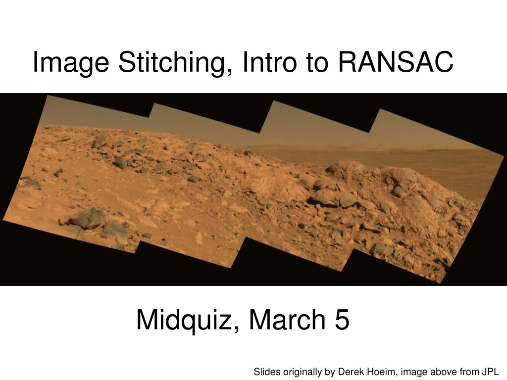
Image Stitching, Intro to RANSAC • Midquiz, March 5 Slides originally by Derek Hoeim, image above from JPL
Last Class: Keypoint Matching 1. Find a set of distinctive key- points 2. Define a region around each keypoint A1 B3 3. Extract and normalize the region content A2 A3 B2 B1 4. Compute a local descriptor from the normalized region 5. Match local descriptors K. Grauman, B. Leibe
Last Class: Summary • Keypoint detection: repeatable and distinctive • Local Max (spatially and scale) of feature score • Descriptors: robust and selective • SIFT: spatial histograms of gradient orientation
Today: Image Stitching • Combine two or more overlapping images to make one larger image Add example Slide credit: Vaibhav Vaish
Homography Reminder • p = K [R t] P • p’ = K’ [R’ t’] P’ • t=t’=0 • p‘=Hpwhere H = K’ R’ R-1 K-1 • Typically only R and f will change (4 parameters), but, in general, H has 8 parameters . X x x' f f'
Views from rotating camera Camera Center
Image Stitching Algorithm Overview • Detect keypoints • Match keypoints • Estimate homography with four matched keypoints (using RANSAC) • Project onto a surface and blend
Image Stitching Algorithm Overview • Detect/extract keypoints (e.g., DoG/SIFT) • Match keypoints (most similar features, compared to 2nd most similar) • Compute Homography. • Declare Success
Homography math reminder: Hp = p’ Write out the lines of this matrix equation. And remember which variables are unknown. Computer Vision, Robert Pless
Ax=b Matlab: x = A\b Then make your homographymatrix H by rearranging x into a 3 x 3 matrix Computer Vision, Robert Pless
Computing homographies in the real world • Assume we have matched points with outliers: How do we compute homographyH? Automatic Homography Estimation with RANSAC
Computing homography • Assume we have matched points with outliers: How do we compute homographyH? Automatic Homography Estimation with RANSAC • Choose number of samples N • Choose 4 random potential matches • Compute H • Project points from x to x’ for each potentially matching pair: • Count points with projected distance < t • E.g., t = 3 pixels • Repeat steps 2-5 N times • Choose H with most inliers How many samples do we need? HZ Tutorial ‘99
Reprise: Automatic Image Stitching • Compute interest points on each image • Find candidate matches • Estimate homographyH using matched points and RANSAC with normalized DLT • Project each image onto the same surface and blend
Choosing a Projection Surface Many to choose: planar, cylindrical, spherical, cubic, etc.
Planar Mapping x x f f For red image: pixels are already on the planar surface For green image: map to first image plane
Planar vs. Cylindrical Projection Planar Photos by Russ Hewett
Spherical Mapping x x f f For red image: compute h, theta on cylindrical surface from (u, v) How can you do this from the homography equation?
Cylindrical Mapping x x f f For red image: compute h, theta on cylindrical surface from (u, v) How can you do this from the homography equation?
Planar vs. Cylindrical Projection Planar Photos by Russ Hewett
Planar vs. Cylindrical Projection Cylindrical
Stitching bigger sets of images together. • … or the incredible beauty of associative groups
Recognizing Panoramas Brown and Lowe 2003, 2007 Some of following material from Brown and Lowe 2003 talk
Recognizing Panoramas Input: N images • Extract SIFT points, descriptors from all images • Find K-nearest neighbors for each point (K=4) • For each image • Select M candidate matching images by counting matched keypoints (M=6) • Solve homographyHij for each matched image
Recognizing Panoramas Input: N images • Extract SIFT points, descriptors from all images • Find K-nearest neighbors for each point (K=4) • For each image • Select M candidate matching images by counting matched keypoints (M=6) • Solve homographyHij for each matched image • Decide if match is valid (ni > 8 + 0.3 nf ) # keypointsin overlapping area # inliers
RANSAC for Homography Initial Matched Points
RANSAC for Homography Final Matched Points
Recognizing Panoramas (cont.) (now we have matched pairs of images) • Find connected components
What’s left? Fancier blending (really a graphics problem ) • Gain compensation: minimize intensity difference of overlapping pixels • Blending • Pixels near center of image get more weight • Multiband blending to prevent blurring
Multi-band Blending (Laplacian Pyramid) • Burt & Adelson 1983 • Blend frequency bands over range l
Capturing Panoramic Images • Tripod vs Handheld • Help from modern cameras • Leveling tripod • Gigapan • Or wing it • Image Sequence • Requires a reasonable amount of overlap (at least 15-30%) • Enough to overcome lens distortion • Exposure • Consistent exposure between frames • Gives smooth transitions • Manual exposure • Makes consistent exposure of dynamic scenes easier • But scenes don’t have constant intensity everywhere • Caution • Distortion in lens (Pin Cushion, Barrel, and Fisheye) • Polarizing filters • Sharpness in image edge / overlap region
Pike’s Peak Highway, CO Photo: Russell J. Hewett Nikon D70s, Tokina 12-24mm @ 16mm, f/22, 1/40s
Pike’s Peak Highway, CO Photo: Russell J. Hewett (See Photo On Web)
360 Degrees, Tripod Leveled Photo: Russell J. Hewett Nikon D70, Tokina 12-24mm @ 12mm, f/8, 1/125s
Howth, Ireland Photo: Russell J. Hewett (See Photo On Web)
Handheld Camera Photo: Russell J. Hewett Nikon D70s, Nikon 18-70mm @ 70mm, f/6.3, 1/200s
Handheld Camera Photo: Russell J. Hewett
Les Diablerets, Switzerland Photo: Russell J. Hewett (See Photo On Web)
Macro Photo: Russell J. Hewett & Bowen Lee Nikon D70s, Tamron 90mm Micro @ 90mm, f/10, 15s
Side of Laptop Photo: Russell J. Hewett & Bowen Lee