Download
1 / 67
670 likes | 814 Views
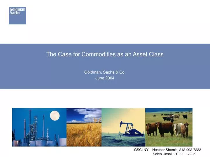
The Case for Commodities as an Asset Class Goldman, Sachs & Co. June 2004. GSCI NY – Heather Shemilt, 212-902-7222 Selen Unsal, 212-902-7225. Executive Summary GSCI: The Portfolio Diversifier; The Portfolio Enhancer.

E N D
The Case for Commodities as an Asset ClassGoldman, Sachs & Co.June 2004 GSCI NY – Heather Shemilt, 212-902-7222 Selen Unsal, 212-902-7225
Executive SummaryGSCI: The Portfolio Diversifier; The Portfolio Enhancer A broadly diversified, long only, passive investment in the commodity markets provides investors with significant benefits • Counter-cyclical with Stocks and Bonds: • Commodities are significantly negatively correlated with both Bonds and Equities, implying that even a small allocation to commodities will reduce portfolio volatility. • High Returns: • The GSCI historically has had high equity-like returns: +12.24% per annum (1 Jan 1970 - 31 May 2004) • GSCI returns can be exceptional: + 41% in 1999, + 50% in 2000, +32% in 2002, +20% in 2003 • Inflation Hedge: • The GSCI provides a hedge against rising inflation, even when inflation is rising from a low base. • Diversification When You Need it Most: • The GSCI has the largest positive impact on a financial portfolio when financial assets have their worst returns. During these “hostile markets”, equities and bonds tend to fall together and provide little diversification. Goldman Sachs recommends a strategic allocation to commodities as a separate asset class to hedge macroeconomic risk, decrease expected portfolio risk and to increase expected portfolio returns. Investor participation in the commodity markets has grown significantly in the last 10 years.
Estimated Global GSCI Investment Growth Investment Soars in 1Q04 We estimate that there is currently $20 billion benchmarked to the GSCI USD 2004YTD 1991 1992 1993 1994 1995 1996 1997 1998 1999 2000 2001 2002 2003 Source: Goldman Sachs
Table of Contents • What is the GSCI? • The Strategic Case • Commodity Returns: Tied to the Business Cycle • Where Commodity Returns Come From • Energy Drives Diversification • How to Invest • Appendix • Liquidity • The Case for Long Run Returns 3
What is the GSCI? Composition of the GSCI as of May 31, 2004 • The GSCI is designed to provide investors with a reliable and publicly available benchmark for investment performance in the commodity markets comparable to the S&P 500 or FT equity indices. • The GSCI has become the premier global commodity benchmark for institutions making allocations to commodities. • The GSCI is a world-production weighted index, the analogue to market capitalization weighting for equities. Precious Metals Livestock 2.08% 6.85% Industrial Metals The GSCI was created in 1991 and the Index based at 100 in 1970 The GSCI futures and options contracts were listed on the CME in July 1992 6.96% Agriculture Energy 15.46% 68.64% • The GSCI has a Futures and an Optionscontractlisted on the Chicago Mercantile Exchange (CME) since July 1992. • The GSCI Excess Return Index tracks an investment in a basket of world-production weighted nearby commodity futures. The index assumes you are always invested in nearby futures contracts. Therefore it is calculated by rolling forward your first nearby contracts into the next nearby contracts mechanically on the 5th-9th business day of each month using the official closing futures prices. • The GSCI Total Return Indextracks a fully collateralized investment. In addition to tracking the rolling investment of nearby futures, it assumes for every dollar you have invested in futures you have a corresponding dollar invested in 3 month USD Tbills. • The rules and regulations governing the GSCI are overseen by an 8 person Policy Committee including members from PGGM Pension, Government of Singapore Investment Corp, The Harvard Business School, and The Chicago Mercantile Exchange. Reuters Page : GSCI Bloomberg : GSCI <go> Source: Goldman Sachs
Goldman Sachs Commodity Index Composition The broad range of commodities provides the GSCI with a high level of diversification. The production weights are based on the average quantity of production in the last five years of available data. Production weighting provides the GSCI with significant advantages, both as an economic indicator and as a measure of investment performance.
Who Invests in the GSCI? BelgiumCanadaDenmarkFinlandFranceGermany Hong KongItalyLuxembourgNetherlandsNorwaySaudi ArabiaSingaporeSpainSwedenSwitzerland UKUS etc... Pension Funds Foundations and Endowments High Net-Worth Individuals Insurance Companies Asset Managers Hedge Funds Private Banks GSCI was introduced over 13 years ago - we now have investors of all types in over 20 countries and the number is growing
Policy Committee • Goldman Sachs has established a Policy Committee to assist it in connection with the operation of the GSCI. • The Policy Committee currently has 8 members including numerous external investment managers. • The Policy Committee meets on an annual basis and at other times at the request of Goldman Sachs. The principal purpose of the Policy Committee is to advise Goldman Sachs with respect to, among other things, the calculation of the GSCI, the effectiveness of the GSCI as a measure of commodity futures market performance and the need for changes in the composition or methodology of the GSCI. Committee Advisors: Policy Committee members: Jelle Beenen Manager Commodities and Quantitative Strategies Investments PGGM Chia Tai Tee Assistant Director, Investment Policy and Strategy GIC Stuart Porter Vice President, Portfolio Management Harvard Management Co Kenneth A. Froot Andre R. Jakurski Harvard Business School Professor of Finance Oliver Frankel Committee Advisor Managing Director Goldman, Sachs & Co. Heather Shemilt Committee Coordinator Managing Director Goldman, Sachs & Co. David Gilberg Legal Advisor Sullivan & Cromwell Gary Cohn Chairman of the Committee Managing Director Goldman, Sachs & Co. Steven Strongin Managing Director Goldman, Sachs & Co. Laurie Ferber Managing Director Goldman, Sachs & Co. Richard Redding Director Chicago Mercantile Exchange
Asset Class Annual Returns 1970 – May 2004 The Strategic Case: Why Clients Have Commodities In Their Portfolio • GS recommends a permanent strategic holding in commodities as a 'separate asset class' to hedge macroeconomic risk, decrease expected portfolio risk and increase expected portfolio returns. • Commodities are significantly negatively correlated with both Bonds and Equities. This implies that the volatility of a portfolio can be significantly decreased even by allocating only a small percentage of the portfolio to commodities. • The GSCI historically has had high equity-like returns (12.24% per annum since 1970 as of May 31, 2004). • Commodities perform best when other assets perform worst. The GSCI has the largest positive impact on a financial portfolio when financial assets have their worst returns. During these “hostile markets”, equities and bonds tend to fall together and provide little diversification. • The GSCI provides a hedge against rising inflation. Commodities are the only asset class we have found that performs well when inflation is rising, even from a low base. Other traditional inflation hedges only perform well when inflation is high and rising. Commodities offer the best macroeconomic hedge against stronger growth. • Commodities, in sharp contrast to more traditional financial assets, are more directly tied to • current economic conditions. As a result, they tend to generate their best returns in periods of • high economic activity and worst returns in periods of low activity. Thus, we find that as the • level of economic activity rises, the expected returns for financial assets fall, while the • expected returns for commodities rise. 14% 12.24% 12% 11.08% 8.39% 10% 8% 6% 4% 2% 0% 1st Qtr 2nd Qtr 3rd Qtr GSCI SP500 GBond Source: Goldman Sachs.
(-0.09) (-0.10) (-0.10) (-0.14) (-0.18) (-0.18) (-0.20) (-0.22) (-0.22) (-0.23) (-0.23) (-0.26) (-0.26) (-0.29) (-0.30) (-0.37) US Canada Japan France Germany Netherlands Switzerland UK Negative CorrelationGSCI Correlation with Global Financial AssetsDec 1987 - Dec 2003 Quarterly Correlations The GSCI is significantly negatively correlated with financial assets (both bonds and equities). Most importantly, the GSCI has the largest positive impact on a financial portfolio when financial assets have their worst returns. Correlation between GSCI and Bonds Correlation between GSCI and Stocks Correlations between quarterly returns of the GSCI in local currency and the financial asset. For bonds: JPM Total Return Government Bond Index of the respective country in local currency. Exception: for Switzerland the returns of 10y SWAP were converted into total returns. For Equity: S&P500 Total Return Index, Toronto 300TR, Nikkei 225, CAC 40, DAX, Amsterdam Stock Exchange Index (AMS), SBC Index & Zurich Stock Exchange Index (SMI), FTSE - UK all share. Source: Goldman Sachs.
High Equity-Like ReturnsAsset Class Performance 1970 – Mar 2003 The GSCI historically has had high equity-like returns (12.07% per annum since 1970 as of 31Mar04). These high returns coupled with the negative correlation have historically meant that adding commodities to a balanced portfolio not only lowers the overall portfolio volatility but at the same time increases the overall portfolio return. The efficiency, or Sharpe Ratio, is improved significantly. Asset Class Cumulative Returns Asset Class Annual Returns 6000 GSCI Total Return 5000 S&P500 TR US Bonds TR 4000 12.07% 11.15% 8.54% 3000 2000 1000 0 -1000 GSCI SP500 GBond 1Jan70 1Jan75 1Jan80 1Jan85 1Jan90 1Jan95 31Mar04 Source: JP Morgan US Government Bond Index for Gbond, S&P500 Total Return Index for S&P500 and GSCI Total Return Index for GSCI. Asset Class Annual Volatility The Effect of adding GSCI to a 60/40 Stock/Bond Portfolio GSCI added at the Expense of Bonds % GSCI Returns Volatility Sharpe Ratio 19.53% 0% 10.82% 12..15% 0.37 5% 11.04% 11.60% 0.40 10% 11.27% 11.16% 0.44 15% 11.50% 10.82% 0.47 20% 11.72% 10.60% 0.51 25% 11.95% 10.52% 0.53 30% 12.18% 10.56% 0.55 35% 12.40% 10.73% 0.56 40% 12.63% 11.03% 0.57 17.03% 10.48% Note: Portfolio was rebased and geometrically compounded on a quarterly basis. If an efficiency frontier was computed using arithmetic returns, the outcome would have been similar. GSCI SP500 GBond Note: Volatilities are derived from quarterly returns. Source: Goldman Sachs.
60/40 PORTFOLIO INTERNATIONAL EQUITIES SMALL CAP STOCKS AUSTRALIAN EQUITIES CANADIAN EQUITIES NAREIT REAL ESTATE S&P 500 EQUITIES BONDS CASH GSCI Commodities Perform Best When the FinancialPortfolio Performs Worst December 1970 – March 2001 Commodities are negatively correlated to other asset classes and significantly outperform when the portfolio needs diversification most. -7.5% -10.0% -10.7% -16.8% -8.4% -6.5% -12.3% -0.4% 7.4% 32.9% -30.0% -20.0% -10% 0% 10.0% 20.0% 30.0% 40.0% We reviewed returns for a typical 60/40% balanced portfolio for Dec 1970-March 2001. From this period we looked at the periods when the portfolio posted its 10% worst returns and plotted the returns for other assets during those same periods. Source: GS Research
Efficiency Frontier Risk / Return Analysis of a Balanced Portfolio (60% equities / 40% fixed income) whilst Adding in GSCI on a Pro-Rata Basis. (Note: quarterly data from 31-Dec-1969 to 31-Mar-03) Viewed in a portfolio context, a GSCI investment can increase returns and reduce volatility at the same time. 13.00% 100% GSCI 12.50% 12.00% Annualized Return (%) 11.50% 32% GSCI 11.00% 10% GSCI 60 / 40 Portfolio 10.50% 6.00% 8.00% 10.00% 12.00% 14.00% 16.00% 18.00% 20.00% 22.00% Risk (Annualized standard deviation, in %) Source: Goldman Sachs.
NBER- NBER- defined defined cyclical cyclical peak peak Commodities: Firmly Tied to the Business CycleGSCI Relative to U.S. Stocks and Bonds A lack of investment in commodity infrastructure over the past 5 years, driven primarily by significant over-investment in the technology and telecommunication sectors, has resulted in substantial capacity constraints which are already resulting in much higher commodity returns much earlier in the business cycle. Total Return Basis: 1Q70– 1Q04 NBER- defined NBER- cyclical peak defined 550 cyclical peak 500 450 400 350 300 250 200 150 100 50 0 1 Jan 70 1 Jan 74 1 Jan 78 1 Jan 82 1 Jan 86 1 Jan 90 1 Jan 94 1 Jan 98 31 Mar 04 GSCI relative to S&P 500 GSCI relative to Bonds Source Bonds: Ibbotson U.S. government bond series through December 1993; JP Morgan world bond index from December 1993 to present Source US Stocks: Ibotson, S&P.
Spare Capacity, Spare Capacity, Tight Capacity, Tight Capacity, Falling Growth Fast Growth Fast Growth Falling Growth +2 Bonds Equities Commodities Bonds +1 Cash Bonds Equities Commodities 0 Equities Commodities Bonds Cash -1 Cash Commodities Cash Equities -2 = Best-Performing Asset Classes Commodity Returns: Tied to the Business Cycle Both equities and bonds (international and domestic) tend to perform best when economic conditions are worst and the potential for improvement is highest; and tend to perform worst when the economy is strong and there is the greatest potential for negative surprises. Commodities, in sharp contrast to more traditional financial assets, are more directly tied to the current economic conditions. As a result, they tend to perform best in periods of high economic activity and worst in periods of low activity. Thus we find that as the level of economic activity rises, the expected returns for financial assets fall, while the expected returns for commodities rise. • The chart depicts the business cycle in terms of the Global Output Gap (When Actual GDP exceeds Potential GDP) • Please note that the 4 business cycle periods above are not equal in duration.
60Eq/30FI/10 57Eq/38FI/5 60Eq/40FI GSCI Comm Comm Annualized Return 10.50% 11.85% 11.17% 10.82% Standard Deviation 12.26% 19.81% 11.22% 11.69% Sharpe Ratio 33.76% 27.69% 42.80% 38.09% Annual returns of 60/40 <0% -5.72% 14.52% -4.22% -4.38% Annual returns of 60/40 <-5% -11.13% 47.72% -7.46% -8.52% Exceptional GSCI Returns When You Need It Most • The highlighted rows indicate years in which a 60% Equity/ 40% Bond Portfolio exhibits negative returns. • In these years when the financial portfolio exhibits negative returns the GSCI typically exhibits strong returns and provides diversification when you need it most.
An Investment in the GSCI is Not Only an Investment in Commodity Prices GSCI Spot Index Jan 1970 – May 2004 An investment in commodities is NOT only an investment in the change in commodity prices. Commodity prices have been highly cyclical, historically generating annualized returns of only 3.26% from 1Jan70 to 31May04. 320 300 280 260 240 220 200 180 160 140 GSCI Spot Index 120 100 80 1 Jan 70 1 Jan 75 1 Jan 79 1 Jan 83 1 Jan 87 1 Jan 91 1 Jan 95 1 Jan 99 31 May 04 Source: Goldman Sachs.
An Investment in Commodity Returns has Historically Exhibited High Equity-Like Returns Historically, the GSCI Total Return Index has exhibited excellent returns (i.e. 12.24% annualized returns from Jan 1, 1970 – May 31, 2004) Meanwhile, the GSCI Spot Index, which simply measures the changes in commodity prices, has only returned a mere 201.41% since the index was based at par in 1970 (3.26% annualized returns) GSCI Total Return vs. GSCI Spot Return: Jan 1970 – May 2004 5500 5000 4500 GSCI Total Return Index 4000 3500 3000 2500 2000 1500 GSCI Spot Index 1000 500 0 1 Jan 70 1 Jan 74 1 Jan 78 1 Jan 82 1 Jan 86 1 Jan 90 1 Jan 94 1 Jan 98 31 May 04 Source: Goldman Sachs.
403 Forward Price = spot + interest rate + storage cost - borrowing cost Gold Price 400 1 month Spot Term Contango“Normal” Upwardly Sloped Forward Curve In commodity markets the “full carry” forward price curve represents only the upper limit that prices can trade at. Key to commodity market returns is that the forward market price does not have to trade at the “full carry” fair forward price (as they must in financial markets) . As detailed in the example to the right, they will not trade higher than the fair forward price but they can and regularly do trade at a substantial discount to the fair forward price. Indeed the forward prices often trade below spot prices (which is referred to as backwardation) Just like financial assets, you can calculate the “full carry” fair forward price of a commodity: Financial Formula: Spot Price + Interest Rate – Borrowing Costs – Dividend/Coupon = Full Carry Fair Forward Price Commodity Formula: Spot Price + Interest Rate – Borrowing Costs + Storage Costs = Full Carry Fair Forward Price In the case of stocks and bonds, the “full carry” forward price must be the equal to the forward price, otherwise there is an arbitrage opportunity. Commodities, on the other hand, regularly do not trade at the ‘full carry” forward price. However note that like financial markets they can not trade higher than the “full carry” forward price. E.g.. suppose that gold is trading at $400 and it’s fair value forward price is $403. If gold trades higher than $403 (e.g. $403.10) an arbitrage opportunity exists. I.e. you could buy spot gold at $400 and then sell forward at 403.10 locking in a minimum $0.10 per oz profit (your costs include the interest paid to borrow the $$ to finance the purchase today plus storage fees; profit is the difference you sell it for above those costs)
Spot Price Forward Price Forward Price Spot Price Backwardated Forward Curves: Commodities are Different The returns from holding physical commodities do NOT equal the returns from a GSCI-style investment. A GSCI-style investment is an investment that tracks the returns from: 1. being invested in front month futures 2. rolling forward those futures each month on the 5th to 9th business day, just prior to expiration of the contract. Convenience Yield: The market often pays a premium for readily available commodities and this is reflected in an inverted (backwardated) forward price curve. This backwardation can be exaggerated given that: Commodities are often not borrowable. Commodities are often difficult to store. When forward prices are below spot prices, commodity investment returns are significantly higher than the change in spot prices. Unlike in contango markets, there is no limit to the degree of backwardation that can prevail in commodity markets. Backwardation Contango
Theoretically: Why Should Commodities Generate Long Run Returns? The Keynes Argument The Future of Commodity Returns Does Not Depend on the Long-term Outlook for Commodity Prices. Commodity Returns are Based on Real Economics and Depend on the Balance Between Supply and Demand for Risk Capital in the Commodity Markets. • Investor Capital in Financial and Commodity Markets • Investors providing capital to equity and fixed income markets are providing capital for ongoing operations of a particular enterprise and returns are generated by the ongoing viability of that enterprise. • Investors in commodity markets do not directly provide capital to the commodity producers. • Instead, the investors long positions in commodity futures allows the producing firms to externalise their short-term commodity price risk via hedging (ie. The commodity producers take the short side of the futures). This hedging activity allows the producers to better utilise their existing capital. • Commodity hedging is key to the commodity producers business by allowing the firm to separate its business risk - the ability to produce at low cost and market desirable products (the core function of equity risk-capital) from its commodity price risk.
$40.00 $38.00 $38 June July August Fundamentally: Why Should Commodities Generate Long Run Returns? The Shortage Dynamic and Oil Returns When inventories are low relative to demand, the market is vulnerable to temporary front month price spikes. In the oil market, you can often get unexpected surges in demand (due to cold weather, increased transport demand, etc.) or disruptions in supply (due to weather problems, political disruption or maintenance breakdown). When there is an insufficient “buffer” of inventories, front month prices can move up sharply. Oil Price ($ barrels)
Returns from Rolling Futures Contracts in the Oil Market The WTI Crude Oil Excess return index measures an investment in front month crude oil rolled forward each month to the next nearby contract keeping you continuously invested in prompt oil futures, and thereby allowing you to take maximum advantage of potential backwardation. Investment returns, as measured by the oil excess return index can be substantially higher than oil spot price changes. The cumulative effect of backwardation due to temporary price spikes can produce substantial returns. Prices do not need to be trending upwards to produce substantial returns. Jan 1996 - Apr 1997 125 +101% 100 GS Crude Oil Excess Return Index +50% 75 50 +34% % Change Crude Oil Price 25 +0% 0 Oil prices return to starting level -25 1Jan96 1Mar96 1May96 1Jul96 1Sep96 1Nov96 1Jan97 1Apr97 Jan 2000 - Dec 2000 100 +85% 80 GS Crude Oil Excess Return Index 60 % Change +42% +38% 40 20 +5% Crude Oil Price 0 -20 1Jan00 1Mar00 1May00 1Jul00 1Sep00 1Nov00 31Dec00 Jan 2003 – Dec 2003 40 +26.2% GS Crude Oil Excess Return Index 30 20 10 % Change +4.2% 0 Crude Oil Price -10 -20 31Dec02 1Mar03 1May03 1Jul03 1Sep03 1Nov03 31Dec03 Source: Goldman Sachs.
Temporary Price Spikes Create Significant Backwardation In a GSCI-style investment, the investor can capitalize on front month price spikes. Here, for example, the market is willing to pay a premium for “front month oil” to satisfy an immediate need for that commodity. When demand is strong and inventories are scarce, the front end of the curve can steepen into extreme backwardation very quickly. This allows the investor to sell his long position substantially above the one month forward price where he re-establishes the position. The investor earns significant returns from price spikes, even if those spikes are temporary. 1996 Mar 19: front-month spread = $3.51 backwardation 28 26 Oil Price in $/Barrel 24 22 20 18 Mar 11: front–month spread = $0.80 backwardation 16 1Jan96 1Mar96 1May96 1Jul96 1Sep96 1Nov96 31Dec96 WTI Price 11mar96 Fwd Curve 19mar96 Fwd Curve 2000 June 20: front-month spread = $2.40 backwardation 38.00 35.86 Oil Price in $/Barrel 33.71 31.57 29.43 27.29 June 7: front-month spread = $0.67 backwardation 25.14 23.00 1Jan00 1Apr00 1Jul00 1Sep00 1Nov00 31Dec00 WTI Price 7jun00 Fwd Curve 20jun00 Fwd Curve 2003 40.00 Feb 12: front-month spread = $1.32 backwardation Feb 3: front-month spread = $0.60 backwardation 37.50 35.00 32.50 Oil Price in $/Barrel 30.00 27.50 25.00 1Jan03 1Feb03 1Apr03 1May03 1Jun03 1Jul03 1Aug03 1Oct03 1Nov03 31Dec03 WTI Price 03Feb03 Fwd Curve 14Feb03 Fwd Curve Source: Goldman Sachs.
40 350 Phase I Phase II At the beginning of a 340 commodity rally, stocks 35 draw and price levels appreciate 330 30 320 Once stocks are 25 310 exhausted, volatility increases WTI Prices 300 significantly (left axis) 20 290 15 US Crude Oil Inventories 280 (right axis) 10 270 Jan-99 Mar-99 May-99 Aug-99 Oct-99 Dec-99 Feb-00 May-00 Jul-00 Sep-00 Dec-00 The 2 Phases of a Commodity Price Rally $/bbl (left axis); million barrels (right axis)
400 Phase I Phase II 350 Phase I generated 102% returns 300 250 200 Phase II generated an additional 174% returns 150 through November 2000 100 50 Jan-99 Mar-99 May-99 Aug-99 Oct-99 Dec-99 Feb-00 May-00 Jul-00 Sep-00 Dec-00 Significant Returns Follow in Phase II GSEN Index: Jan 99 =100
Returns from Rolling Futures Contracts in the Oil Market Jan 2003 – Dec 2003 40 The WTI Crude Oil Excess return index measures an investment in front month crude oil rolled forward each month to the next nearby contract keeping you continuously invested in prompt oil futures, and thereby allowing you to take maximum advantage of potential backwardation. Prices do not need to be trending upwards to produce substantial returns. +26.2% 30 GS Crude Oil Excess Return Index 20 10 +4.2% 0 % Change -10 Crude Oil Price -20 31Dec02 1Mar03 1May03 1Jul03 1Sep03 1Nov03 31Dec03 Source: Goldman Sachs.
When to Buy Commodities Rather Than Commodity Related Stocks Based on a view of the commodity, a direct investment (eg via the GSCI) is the preferred investment vehicle. Direct commodity investments provide substantial additional returns during periods of shortage relative to to equity investments. OSX = Philadelphia Stock Exchange Oil Service Sector Index Rolling 1-month WTI futures Rolling 12-month 240 (+110%) WTI futures (+68%) 220 200 180 Buy and Hold Mar-04 WTI futures contract (+56%) 160 140 120 OSX (+9%) 100 80 Jul-03 Jul-02 Oct-03 Apr-02 Apr-03 Jun-03 Oct-02 Jan-02 Jun-02 Jan-03 Nov-03 Dec-03 Aug-03 Sep-03 Mar-02 Mar-03 Feb-02 Feb-03 Nov-02 Dec-02 Aug-02 Sep-02 May-03 May-02
Backwardation of the GSCIJanuary 1995 – May 31, 2004This graph represents the percentage backwardation or contango between the 1st and 2nd month futures contracts on the GSCI 7 The GSCI futures contract has been in backwardation 50% of the time. However, note that there is no limit to backwardation. Contango, meanwhile, is limited to the “full carry” fair forward (i.e. the spot price plus financing and storage costs) 6 Backwardation The Venezuelan supply shock coupled with the lack of spare capacity resulted in the market returning quickly to backwardation in ’02 and ‘03 5 4 1999: fundamentals begin to shift; demand exceeds supply and as inventories are depleted, the market begins to move to backwardation 3 2 GSCI Front Month Backwardation (%) 1 0 - 1 - 2 Contango - 3 1998: oil market is oversupplied contango results Recession (poor demand) and contango returns - 4 1 Jan 95 1 Jan 96 1 Jan 97 1 Jan 98 1 Jan 99 1 Jan 00 1 Jan 01 1 Jan 02 1 Jan 03 31 May 04 % Backwardation / Contango Source: Goldman Sachs Research
Investment Returns in the Commodity MarketsGSCI Excess Return Index and Projected ReturnsJan02 – Dec02 If we only looked at the 1.36% contango that existed in the commodity market on 31Dec,01 and extrapolated that forward, it would have suggested a –16.33% negative return by the end of Dec02. In fact, the GSCI Excess Return Index was up 29.92% at the end of Dec02. The best prediction of the forward return will be one based on the determination of the fundamental supply / demand equilibrium One can not predict the investment return by simply looking at the shape of the curve on any one day. 35 GSCI Excess Return 30 25 Contango on 31Dec01: -1.36% 20 15 Actual Return: GSCI Excess Return Index up 29.92% at 31Dec02 10 5 0 Projected movement based on contango on 1 Nov: - 1.36% per month, i.e. –16.33% by end of Dec 02. -5 -10 -15 -20 1Jan02 1Mar02 1May02 1Jul02 1Sep02 1Nov02 31Dec02 Source: Goldman Sachs.
Backwardation in WTI Crude OilMarch 1983* – May 31, 2004 (*WTI futures first started trading in March 83)This graph represents the percentage backwardation or contango between the 1st and 2nd month futures contracts for NYMEX WTI Crude Oil Since inception of NYMEX WTI Crude Oil futures, the contract has been in backwardation 66% of the time delivering an average yield of 0.76% per month. Crude Backwardation 20 15 10 5 Crude Front Month Backwardation (%) 0 - 5 - 10 - 15 31 Mar 83 1 Jan 86 1 Jan 88 1 Jan 90 1 Jan 92 1 Jan 94 1 Jan 96 1 Jan 98 1 Jan 00 1 Jan 02 31 May 04 % Backwardation / Contango Source: Goldman Sachs
Backwardation is not a Temporary Phenomenon From the inception of NYMEX WTI Crude Oil futures, to 31 May 2004, WTI has been in backwardation 66% of the time. Source: Goldman Sachs.
Standard Deviation vs. Mean Returns for GSCI, GS Energy, GS Non-Energy, Equities, and Bonds The GS Energy Sub-index generates higher average returns than the overall GSCI, the GS Non-Energy Sub-index, equities and bonds. Importantly, despite higher volatility, on a risk-reward basis the GS Energy Sub-index substantially outperforms the Non-Energy Sub-index. 20% Annualized standard deviation of monthly returns - horizontal axis vs. GSEN 18% Annualized average monthly returns - vertical axis 17.6% (Jan 1987 - Dec 2003) 16% 14% S&P 500 12% 11.4% 10% GSCI 11.2% US GBond 8% 7.9% 6% GSNE Higher total returns are needed to compensate financial 4.7% 4% investors for bearing the risk of taking long positions in volatile commodity markets. 2% 0% 0% 5% 10% 15% 20% 25% 30% 35% Source: Goldman Sachs
Correlation between GSCI and GS Sub-indices to SP500 Monthly Observations GS Energy Sub-index returns are negatively correlated with S&P 500 returns, providing diversification benefits to investors. In contrast, Non-energy Sub-index returns are positively correlated with equity returns. Precious Metals are also negatively correlated but have the lowest return profile of all the sub-indices & therefore offer little portfolio diversification Source: Goldman Sachs
Correlation between GSCI and GS Sub-indices to SP500 Quarterly Observations GS Energy Sub-index returns are negatively correlated with S&P 500 returns, providing diversification benefits to investors. In contrast, Non-energy Sub-index returns are positively correlated with equity returns. Precious Metals are also negatively correlated but have the lowest return profile of all the sub-indices & therefore offer little portfolio diversification GSCI Industrial Metals GSCI Precious Metals GSCI Livestock GSCI Non-Energy GSCI Energy GSCI Agriculture GSCI Source: Goldman Sachs
Performance of the GSCI Energy Sub-Index by Economic Environment (Jan 1987-Dec 2003) Monthly changes in US IP RISING FALLING Average Return 32.17% 22.52% ABOVE Standard Deviation of returns 37.11% 25.88% US IP relative to trend Sharpe Ratio 0.87 0.87 Average Return 7.94% -2.97% BELOW Standard Deviation of returns 26.11% 28.78% Sharpe Ratio 0.30 -0.10 Performance of the GSCI Index by Economic Environment (Jan 1987-Dec 2003) Monthly changes in US IP RISING FALLING Average Return 17.85% 10.27% ABOVE Standard Deviation of returns 20.70% 15.21% US IP relative to trend Sharpe Ratio 0.86 0.68 Average Return 9.04% -3.18% BELOW Standard Deviation of returns 15.28% 18.16% Sharpe Ratio 0.59 -0.17 Performance of the GSCI Non-Energy Sub-Index by Economic Environment (Jan 1987-Dec 2003) Monthly changes in US IP RISING FALLING Average Return 2.53% -4.07% ABOVE Standard Deviation of returns 9.64% 8.98% US IP relative to trend Sharpe Ratio 0.26 -0.45 Average Return 10.38% 0.23% BELOW Standard Deviation of returns 9.13% 8.93% Sharpe Ratio 1.14 0.03 Risk and Reward Statistics by Macro Environment Monthly Observations: Industrial Production Level and Change Relative to Trend The GS Energy Sub-index outperforms the overall index on a risk reward basis when macro-economic activity is above trend. Source: Goldman Sachs
Performance of the GSCI Energy Sub-Index by Economic Environment (1Q1987-4Q2003) G7 Real GDP Growth Relative to Trend RISING FALLING Average Return 24.34% 20.36% G7 Real ABOVE Standard Deviation of returns 30.63% 74.33% GDP Sharpe Ratio 0.79 0.27 Level Relative Average Return 10.54% 3.34% to Trend BELOW Standard Deviation of returns 29.58% 24.34% Sharpe Ratio 0.36 0.14 Performance of the GSCI Index by Economic Environment (1Q1987-4Q2003) G7 Real GDP Growth Relative to Trend RISING FALLING Average Return 20.07% 9.20% G7 Real ABOVE Standard Deviation of returns 15.43% 42.49% GDP Sharpe Ratio 1.30 0.22 Level Relative Average Return 10.36% 1.50% to Trend BELOW Standard Deviation of returns 14.71% 15.25% Sharpe Ratio 0.70 0.10 Performance of the GSCI Non-Energy Sub-Index by Economic Environment (1Q1987-4Q2003) G7 Real GDP Growth Relative to Trend RISING FALLING G7 Real Standard Deviation of returns 12.79% -8.46% ABOVE Standard Deviation of returns 8.43% 8.38% GDP Sharpe Ratio 1.52 -1.01 Level Relative Average Return 5.97% 1.50% to Trend BELOW Standard Deviation of returns 9.45% 15.25% Sharpe Ratio 0.63 0.10 Risk and Reward Statistics by Macro Environment Quarterly Observations: Real GDP Level and Growth Relative to Trend The GS Energy Sub-index outperforms the overall index on a risk reward basis when macro-economic activity is above trend. Source: Goldman Sachs
Swaps Structured Notes Options GSCI Futures Contract Third Party Asset Managers Ways To Invest in the GSCI
1. Implementation via Swaps • Total Return Swap Percentage Change in GSCI Total Return Client Goldman Sachs 3mo T-Bills Per annum hedge management fee • Excess Return Swap Percentage Change in GSCI Excess Return Client Goldman Sachs Per annum hedge management fee
Implementation via Swaps The majority of GSCI investors buy over-the-counter swaps
Implementation via SwapsTotal Return Swaps vs. Excess Return Swaps GSCI Total Return Swaps are recommended over GSCI Excess Return Swaps. • It is important to note that the GSCI Excess Return plus T-bills does not equal the GSCI Total Return because it ignores the impact of the re-investment of T-bill collateral yield back into the commodity investment
2a. GSCI-linked Notes Structured notes are a way to gain commodity exposure but at the same time to limit your downside risk
2b. GSCI Options Options are another way to gain commodity exposure but at the same time to limit your downside risk