Download

1 / 33
360 likes | 501 Views
Root Locus Method. Root Locus. Motivation To satisfy transient performance requirements, it may be necessary to know how to choose certain controller parameters so that the resulting closed-loop poles are in the performance regions, which can be solved with Root Locus technique. Definition

E N D
Root Locus • Motivation To satisfy transient performance requirements, it may be necessary to know how to choose certain controller parameters so that the resulting closed-loop poles are in the performance regions, which can be solved with Root Locus technique. • Definition A graph displaying the roots of a polynomial equation when one of the parameters in the coefficients of the equation changes from 0 to . • Rules for Sketching Root Locus • Examples • Controller Design Using Root Locus Letting the CL characteristic equation (CLCE) be the polynomial equation, one can use the Root Locus technique to find how a positive controller design parameter affects the resulting CL poles, from which one can choose a right value for the controller parameter.
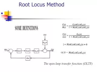
Disturbance D(s) Reference Input R(s) Control Input U(s) + Output Y(s) Error E(s) + + GC (s) Gf (s) - Plant H(s) G(s) Closed-Loop Characteristic Equation (CLCE) • The closed-loop transfer function GYR(s) is: • The closed-loop characteristic equation (CLCE) is: • For simplicity, assume a simple proportional feedback controller: • The transient performance specifications define a region on the complex plane where the closed-loop poles should be located. • Q: How should we choose KP such that the CL poles are within the desired performance boundary? Img. Transient Performance Region Real
Motivation Ex:The closed-loop characteristic equation for the DC motor positioning system under proportional control is: Q: How to choose KP such that the resulting closed-loop poles are in the desired performance region? • How do we find the roots of the equation: as a function of the design parameter KP ? • Graphically display the locations of the closed-loop poles for all KP>0 on the complex plane, from which we know the range of values for KP that CL poles are in the performance region.
Root Locus – Definition Root Locus is the method of graphically displaying the roots of a polynomial equation having the following form on the complex plane when the parameter K varies from 0 to : where N(s) and D(s) are known polynomials in factorized form: Conventionally, the NZroots of the polynomial N(s) , z1 , z2 , …, zNz , are called the finite open-loop zeros. The NProots of the polynomial D(s) , p1 , p2 , …, pNp , are called the finite open-loop poles. Note: By transforming the closed-loop characteristic equation of a feedback controlled system with a single positive design parameter K into the above standard form, one can use the Root Locus technique to determine the range of K that have CL poles in the performance region.
Methods of Obtaining Root Locus • Given a value of K, numerically solve the 1 + K G(s) = 0 equation to obtain all roots. Repeat this procedure for a set of K values that span from 0 to and plot the corresponding roots on the complex plane. • In MATLAB, use the commands rlocus and rlocfind. A very efficient root locus design tool is the command rltool. You can use on-line help to find the usage for these commands. • Apply the following root locus sketching rules to obtain an approximated root locus plot. >> op_num=[0.48]; >> op_den=[0.0174 1 0]; >> rlocus(op_num,op_den); >> [K, poles]=rlocfind(op_num,op_den); No open-loop zeros Two open-loop poles
Root Locus Sketching Rules Rule 1: The number of branches of the root locus is equal to the number of closed-loop poles (or roots of the characteristic equation). In other words, the number of branches is equal to the number of open-loop poles or open-loop zeros, whichever is greater. Rule 2: Root locus starts at open-loop poles (when K= 0) and ends at open-loop zeros (when K=). If the number of open-loop poles is greater than the number of open-loop zeros, some branches starting from finite open-loop poles will terminate at zeros at infinity (i.e., go to infinity). If the reverse is true, some branches will start at poles at infinity and terminate at the finite open-loop zeros. Rule 3: Root locus is symmetric about the real axis, which reflects the fact that closed-loop poles appear in complex conjugate pairs. Rule 4: Along the real axis, the root locus includes all segments that are to the left of an odd number of finite real open-loop poles and zeros. Check the phases
Root Locus Sketching Rules Rule 5: If number of poles NP exceeds the number of zeros NZ , then as K, (NP - NZ) branches will become asymptotic to straight lines. These straight lines intersect the real axis with angles k at 0 . If NZ exceeds NP , then as K0, (NZ - NP) branches behave as above. Rule 6: Breakaway and/or break-in (arrival) points should be the solutions to the following equations:
Root Locus Sketching Rules Rule 7: The departure angle for a pole pi ( the arrival angle for a zero zi) can be calculated by slightly modifying the following equation: The departure angle qjfrom the pole pjcan be calculated by replacing the term with qj and replacing all the s’s with pj in the other terms. Rule 8: If the root locus passes through the imaginary axis (the stability boundary), the crossing point jand the corresponding gain K can be found as follows: • Replace s in the left side of the closed-loop characteristic equation with jw to obtain the real and imaginary parts of the resulting complex number. • Set the real and imaginary parts to zero, and solve for wand K. This will tell you at what values of K and at what points on the jw axis the roots will cross. angle criterion magnitude criterion
Steps to Sketch Root Locus Step 1: Transform the closed-loop characteristic equation into the standard form for sketching root locus: Step 2: Find the open-loop zeros, zi, and the open-loop poles, pi. Mark the open-loop poles and zeros on the complex plane. Use ´ to represent open-loop poles and ¡ to represent the open-loop zeros. Step 3: Determine the real axis segments that are on the root locus by applying Rule 4. Step 4: Determine the number of asymptotes and the corresponding intersection s0 and angles qkby applying Rules 2 and 5. Step 5: (If necessary) Determine the break-away and break-in points using Rule 6. Step 6: (If necessary) Determine the departure and arrival angles using Rule 7. Step 7: (If necessary) Determine the imaginary axis crossings using Rule 8. Step 8: Use the information from Steps 1-7 and Rules 1-3 to sketch the root locus.
qDV qD Ei q KP 0.03 Controller Plant G(s) qV 0.03 Example 1 DC Motor Position Control In the previous example on the printer paper advance position control, the proportional control block diagram is: Sketch the root locus of the closed-loop poles as the proportional gain KP varies from 0 to ¥. Find closed-loop characteristic equation:
Example 1 Step 1: Transform the closed-loop characteristic equation into the standard form for sketching root locus: Step 2: Find the open-loop zeros, zi , and the open-loop poles, pi : Step 3: Determine the real axis segments that are to be included in the root locus by applying Rule 4. K No open-loop zeros open-loop poles
Example 1 Step 4: Determine the number of asymptotes and the corresponding intersection s0 and angles qkby applying Rules 2 and 5. Step 5: (If necessary) Determine the break-away and break-in points using Rule 6. Step 6: (If necessary) Determine the departure and arrival angles using Rule 7. Step 7: (If necessary) Determine the imaginary axis crossings using Rule 8. Could s be pure imaginary in this example?
Img. Axis 30 20 10 0 Real Axis -60 -50 -40 -30 -20 -10 0 -10 -20 -30 Example 1 Step 8: Use the information from Steps 1-7 and Rules 1-3 to sketch the root locus. -57.47 -28.74
Example 2 A positioning feedback control system is proposed. The corresponding block diagram is: Sketch the root locus of the closed-loop poles as the controller gain K varies from 0 to ¥. Find closed-loop characteristic equation: R(s) + Y(s) U(s) K(s + 80) - Controller Plant G(s)
Example 2 Step 1: Formulate the (closed-loop) characteristic equation into the standard form for sketching root locus: Step 2: Find the open-loop zeros, zi , and the open-loop poles, pi : Step 3: Determine the real axis segments that are to be included in the root locus by applying Rule 4. K open-loop zeros open-loop poles
Example 2 Step 4: Determine the number of asymptotes and the corresponding intersection s0 and angles qkby applying Rules 2 and 5. Step 5: (If necessary) Determine the break-away and break-in points using Rule 6.
Imag Axis 40 30 20 10 Real Axis 0 -10 -20 -30 -40 -140 -120 -100 -80 -60 -40 -20 0 Example 2 Step 6: (If necessary) Determine the departure and arrival angles using Rule 7. Step 7: (If necessary) Determine the imaginary axis crossings using Rule 8. Step 8: Use the information from Steps 1-7 and Rules 1-3 to sketch the root locus.
+ R(s) U(s) Y(s) - Controller Plant G(s) Example 3 A feedback control system is proposed. The corresponding block diagram is: Sketch the root locus of the closed-loop poles as the controller gain K varies from 0 to ¥. Find closed-loop characteristic equation:
Example 3 Step 1: Transform the closed-loop characteristic equation into the standard form for sketching root locus: Step 2: Find the open-loop zeros, zi , and the open-loop poles, pi : Step 3: Determine the real axis segments that are to be included in the root locus by applying Rule 4. open-loop zeros No open-loop zeros open-loop poles
Example 3 Step 4: Determine the number of asymptotes and the corresponding intersection s0 and angles qkby applying Rules 2 and 5. Step 5: (If necessary) Determine the break-away and break-in points using Rule 6.
Example 3 Step 6: (If necessary) Determine the departure and arrival angles using Rule 7. Step 7: (If necessary) Determine the imaginary axis crossings using Rule 8. CLCE
Imag Axis 4 3 2 1 Real Axis 0 -1 -2 -3 -4 -6 -5 -4 -3 -2 -1 0 Example 3 Step 8: Use the information from Steps 1-7 and Rules 1-3 to sketch the root locus.
Example 4 Y(s) R(s) A feedback control system is proposed. The corresponding block diagram is: Sketch the root locus of the closed-loop poles as the controller gain K varies from 0 to ¥. Find closed-loop characteristic equation: + U(s) K - Controller Plant G(s)
Example 4 Step 1: Formulate the (closed-loop) characteristic equation into the standard form for sketching root locus: Step 2: Find the open-loop zeros, zi , and the open-loop poles, pi : Step 3: Determine the real axis segments that are to be included in the root locus by applying Rule 4. open-loop zeros open-loop poles
Example 4 Step 4: Determine the number of asymptotes and the corresponding intersection s0 and angles qkby applying Rules 2 and 5. Step 5: (If necessary) Determine the break-away and break-in points using Rule 6. Step 6: (If necessary) Determine the departure and arrival angles using Rule 7. Step 7: (If necessary) Determine the imaginary axis crossings using Rule 8. One asymptote
Example 4 Step 8: Use the information from Steps 1-7 and Rules 1-3 to sketch the root locus. 9.5273j Stability condition 5.6658j -5.6658j -9.5273j
M Root Locus as an Analysis/Design Tool Mechanical system response depends on the location of the system characteristic values, i.e., poles of the system transfer function. Since root locus tells us how the system poles vary w.r.t. a parameter K, we can use root locus to analyze the effect of parameter variation on system performance. Ex: ( Motion Control of Hydraulic Cylinders ) A V C Recall the example of the flow control of a hydraulic cylinder that takes into account the capacitance effect of the pressure chamber. The plant transfer function is: where M is the mass of the load; C is the flow capacitance of the pressure chamber; A is the effective area of the piston and B is the viscous friction coefficient. Q: How would the plant parameters affect the system response ? B qIN
Img. Axis Real Axis Root Locus as an Analysis/Design Tool • Effect of load (M) on system performance: System characteristic equation: Transform characteristic equation into standard form for root locus analysis by identifying the parameter that is to be varied. In this case, the load mass M is the varying parameter: Standard form Varying parameter open-loop zeros open-loop poles Small M: less overshoot and high natural frequency As M increases: larger overshoot and lower natural frequency Think about the settling time
Img. Axis Real Axis Root Locus as an Analysis/Design Tool • Effect of flow capacitance (C) on system performance: System characteristic equation: Transform characteristic equation into standard form for root locus analysis by identifying the parameter that is to be varied. In this case, the flow capacitance C is the varying parameter: Standard form Varying parameter open-loop zeros NO open-loop poles open-loop poles Smaller C (or less compressible fluid): Larger oscillating frequency and overshoot Larger C: smaller oscillating frequency and overshoot
Img. Axis Real Axis Root Locus as an Analysis/Design Tool • Effect of friction (B) on system performance: System characteristic equation: Transform characteristic equation into standard form for root locus analysis by identifying the parameter that is to be varied. In this case, the viscous friction coefficient B is the varying parameter: Standard form Varying parameter open-loop zeros open-loop poles Smaller B: Larger oscillating frequency and overshoot Larger B: smaller oscillating frequency and overshoot settling time?