Download

1 / 54
740 likes | 1.33k Views
Design with Root Locus. Lecture 9. Objectives for desired response. Improving transient response Percent overshoot, damping ratio, settling time, peak time Improving steady-state error Steady state error. Gain adjustment.

E N D
Design with Root Locus Lecture 9
Objectives for desired response • Improving transient response Percent overshoot, damping ratio, settling time, peak time • Improving steady-state error Steady state error
Gain adjustment • Higher gain, smaller steady stead error, larger percent overshoot • Reducing gain, smaller percent overshoot, higher steady state error
Compensator • Allows us to meet transient and steady state error. • Composed of poles and zeros. • Increased an order of the system. • The system can be approx. to 2nd order using some techniques.
Point A and B have the same damping ratio. Starting from point A, cannot reach a faster response at point B by adjusting K. We have pole at A on the root locus, but we want response like at B. Compensator is preferred. Improving transient response
Compensator configulations Cascade Compensator Feedback Compensator The added compensator can change a pattern of root locus
compensator Method of implementing compensator: 1. Proportional control systems: feed the error forward to the plant. 2. Integral control systems: feed the integral of the error to the plant. 3. Derivative control systems: feed the derivative of the error to the plant.
Types of compensator • Active compensator • PI, PD, PID use ofactive components, i.e.,OP-AMP • Require power source • ss error converge to zero • Expensive • Passive compensator • Lag,Leaduse ofpassive components, i.e., R L C • No need of power source • ss error nearly reaches zero • Less expensive
Improving steady-state error (PI) Placing apole at theorigin to increase system order; decreasing ss error as a result!! (a) Original system without compensation (b) Add a pole at the origin but angular contribution at point A is no longer 180
Improving Steady-State Error (PI) Also add a zero close to the pole at the origin. As angular contribution of the compensator zero and pole cancels out, point A is still on the root locus, and the system type has been increased.
Improving Steady-State Error (PI):Example Choose zero at -1 Damping ratio = 0.174 in both uncompensated and PI cases
Improving Steady-State Error (PI) >> z=[1]; >> n=conv([1 3 2],[1 10]); >> sys=tf(z,n) >> sgrid(0.174,[2,10]) >> [k p]=rlocfind(sys)
Improving Steady-State Error (PI) As shown in the figure, the step response of the PI compensated system approaches unity in the steady-state, while the uncompensated system response approaches 1−0.108 = 0.892. The simulation shows that it takes 18 seconds for the compensated system to reach and stay within ±2% of the final value of unity, while the uncompensated system takes about 6 seconds to settle to within ±2% of its final value of 0.892. This is because there is no pole-zero cancelation and the pole not canceled is very close to the origin.
Finding an intersection between damping ratio line and root locus • Damping ratio line has an equation: where a = real part, b = imaginary part of the intersection point, • Summation of angle from open-loop poles and zeros to the point is 180 degrees
Use the formula to get the real and imaginary part of the intersection point and get • Magnitude of open loop system is 1 No open loop zero
Draw root locus with compensator (system order is up by 1--from 3rd to 4th) • Needs complex poles corresponding to damping ratio of 0.174 (K=158.2) • From K, find the 3rd and 4th poles (at -11.55 and -0.0902) • Pole at -0.0902 can do phase cacellation with zero at -1 (3th order approx.) • Compensated system and uncompensated system have similar transient response (closed loop poles and K are aprrox. The same)
PI Controller A compensator with a pole at the origin and a zero close to the pole is called an ideal integral compensator, or PI controller
Lag Compensator Ideal integral compensation: pole is in the origin, requires active network (costly). Real (passive) integral compensation: pole is close to origin (not in the origin), cheaper. (a) Type 1 uncompensated system (b) Type 1 compensated system Type is not increased. What about steady-state error
Example With damping ratio of 0.174, add lag Compensator to improvesteady-state error by a factor of 10
Step I: find an intersection of root locus and damping ratio line (-0.694+j3.926 withK=164.56) Step II:findKp = lim G(s) as s0 (Kp=8.228) Step III:steady-state error =1/(1+Kp)= 0.108 Step IV:want to decrease error down to0.0108 [Kp = (1 – 0.0108)/0.0108 = 91.593] Step V: require a ratio of compensator zero to pole as91.593/8.228 = 11.132 Step VI: choose apole at0.01, the corresponding Zero will be at 11.132*0.01 = 0.111
3rd order approx. for lag compensator (= uncompensated system) making Same transient response but 10 times Improvement in ss response!!!
If we choose acompensator pole at 0.001 (10 times closer to the origin), we’ll get a compensatorzero at0.0111 (Kp=91.593) New compensator: 4th pole is at -0.01 (compared to -0.101) producing a longer transient response.
SS response improvement conclusions • Can be done either by PI controller (pole at origin) or lag compensator (pole closed to origin). • Improving ss error without affecting the transient response. • Next step is to improve the transient response itself.
Improving Transient Response • Objective is to • Decrease settling time • Get a response with a desired %OS (damping ratio) • Techniques can be used: • PD controller (ideal derivative compensation) • Lead compensator
PD controller: Improving transient response System above controlled by a pure gain (P controller) in the forward path has its root locus going through point A for some value of gain K. • Our goal is to speed up the response at A to that at B, while keeping the percent overshoot unchanged. • The above root locus with a P controller cannot go through point B (sum of angles from the open-loop finite poles and zeros to point B is not an odd multiple of 180◦). A solution is to add a (nonzero) zero to the forward path (e.g., PD controller).
PD controller: Improving transient response • Transfer function of the PD controller Gc(s) = K2 s + K1 = K2(s+K1/K2) = K(s+zc) introduces a zero at −zc Into the forward path. • Effect of the added zero: The added zero will contribute to make the sum of angles from the open-loop finite poles and zeros to the desired point (point B) be an odd multiple of 180◦. Note: an added zero has the effect of pushing the root locus to the left while an added pole has the effect of pushing it to the right. • The new root locus can meet the specific transient response (with shorter settling time) by going through point B for some value of gain K.
Ideal Derivative Compensator • So called PD controller • Compensator adds a zero to the system at –Zc to keep a damping ratio constant with a faster response
(a) Uncompensated system, (b) compensator zero at -2 (d) compensator zero at -3, (d) compensator zero at -4 Indicate peak time Indicate settling time
Settling time & peak time: (b)<(c)<(d)<(a) • %OS: (b)=(c)=(d)=(a) • ss error: compensated systems has lower value than uncompensated one cause improvement in transient response always yields an improvement in ss error
Example design a PD controller to yield 16% overshoot with a threefold reduction in settling time
Step I: calculate a corresponding damping ration (16% overshoot = 0.504 damping ratio) • Step II: search along the damping ratio line for an odd multiple of 180 (at -1.205±j2.064) and corresponding K (43.35) • Step III: find the 3rd pole (at -7.59) which is far away from the dominant poles 2nd order approx. works!!!
More details in step II and III Characteristic equation:
Step IV: evaluate a desired settling time: • Step V: get corresponding real and imagine number of the dominant poles (-3.613 and -6.193)
Location of poles as desired is at -3.613±j6.192
Step VI: summation of angles at the desired pole location, -275.6, is not an odd multiple of 180 (not on the root locus) need to add a zero to make the sum of 180. • Step VII: the angular contribution for the point to be on root locus is +275.6-180=95.6 put a zero to create the desired angle
Compensator: (s+3.006) Might not have a pole-zero cancellation for compensated system
Lead Compensation • A PD controller can be approximated with a lead compensator, which is implemented with a passive network. • If the lead compensator pole is farther from the imaginary axis than the compensator zero, the angular contribution of the compensator is still positive and thus approximates an equivalent single zero. • The advantages of a passive lead compensator over an active PD controller are that (1) no additional power supplies are required and (2) noise due to differentiation is reduced. Zeta2-zeta1=angular contribution
Lead Compensation • • The concept behind lead compensation: the difference between 180◦ and the sum of the angles from the uncompensated system’s poles and zeros to the design point (desired pole location) must be the angular contribution required of the compensator. • That is, • q2 −q1 −q3 −q4 +q5 = (2k+1)180◦ • where q2 −q1 = qc is the angular contribution of the lead compensator. Zeta2-zeta1=angular contribution
• The angular contribution qc can be determined from the rays originating from the desired closed-loop pole and terminating at the compensator pole and zero. These rays can be rotated about the desired closed-loop pole and thus different pairs of compensator pole and zero can be used to meet the transient response requirement. • Different possible lead compensators: differences are in the values of the static error constants, the static gain, the difficulty in justifying a second-order approximation when the design is complete, and the ensuing transient response. • For design we arbitrarily select either a lead compensator pole and zero and find the angular contribution at the design point of this pole or zero with the uncompensated system’s open-loop poles and zeros. The difference between this angle and 180◦ is the required contribution of the remaining compensator pole or zero.
Example Design three lead compensators for the system that has30% OS and will reducesettling time down by a factor of 2.
Step I: %OS = 30% equaivalent todamping ratio = 0.358, Ѳ= 69.02 • Step II: Search along the line to find a point that gives 180 degree (-1.007±j2.627) • Step III: Find a corresponding K ( ) • Step IV: calculate settling time of uncompensated system • Step V: twofold reduction in settling time (Ts=3.972/2 = 1.986), correspoding real and imaginary parts are:
Step VI: let’s put a zero at -5 and find the net angle to the test point (-172.69) • Step VII: need a pole at the location giving 7.31 degree to the test point.