Download
1 / 29
290 likes | 370 Views
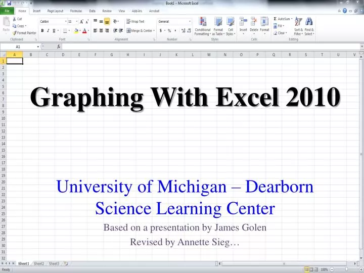
Graphing With Excel 2010. University of Michigan – Dearborn Science Learning Center Based on a presentation by James Golen Revised by Annette Sieg …. Introduction.

E N D
Graphing With Excel 2010 University of Michigan – Dearborn Science Learning Center Based on a presentation by James Golen Revised by Annette Sieg…
Introduction • Before using this module you must already understand the basics of graphing (e.g., identifying dependent and independent variables, plotting data points). • If you need help with basic graphing, please refer to the Graphing Introduction module available from the Science Learning Center.
Getting Started • You’ve collected data from an experiment, and you want to graph your data to see if there is a pattern (i.e., relationship) among the data. Graphing by hand is an option, but using a computer program will make your results more accurate and look more professional. • An overriding principle in graphing, which will be emphasized in this module, was famously identified by Edward Tufte (1983) as,“above all else show the data.” • Tufte (1983) labeled graphical content which merely enlivens the display of data (e.g., extraneous background colors and lines) as “chartjunk” • Default Excel 2010 graphs contain a variety of chartjunk, and you will be encouraged to eliminate it as part of this module.
Getting Started • Please follow along, step-by-step, with Excel 2010 running on your computer as we work through graphing some sample Chemistry experimental data
Getting Started • Open an Excel spreadsheet and begin entering your data. Make sure you have a title for the spreadsheet and column headings for each variable. (Initially, we will only be working with continuous variables) Step 1: Enter your raw data into the spreadsheet. Here, we used column “B” for the independent variable (x-axis), and column “C” for the dependent variable (y-axis).
Graphing Step 2: Highlight the data that you wish to graph. Only the area highlighted will be graphed. So make sure that you have selected all the data that you want to appear on the graph.
Graphing Step 3: • With your data highlighted, select the Insert tab • Under the Charts section of the Insert tab there are several options for different types of graphs. • Initially, we’re going to create a Scatterplot which plots the x- and y-coordinates of each data point without additional colored lines, bars, etc.
Graphing Step 3 cont’d: • Click on the Scatter with only Markers option
Step 4: At this point you have the ‘rough draft’ version of your graph. Excel gives you a default graph that is typically loaded with features you will want to change (e.g., unlabeled axes, gridlines, legend) You can (and should!) edit the graph further by clicking on it and using the features in Chart Tools.
Graph Editing – Labeling Step 5: • In order to label your graph, under Chart Tools, select the Layout tab. • Use the Axis Titles and Chart Title buttons to label your graph appropriately.
Graph Editing – Labeling Step 5 cont’d: When finished with labeling, your graph should look like this.
Graph Editing – Gridlines Step 6: • Typically, graphs do not require the gridlines that are in Excel default graphs. Graphs are used to reveal patterns and relationships among data, and the precise value of each data point — which is demonstrated by gridlines — is usually unnecessary. • One instance when gridlines are useful is in illustrating small differences (e.g., between the height of bars in a bar graph when the bars are of similar height). • In our Scatterplot example, the gridlines do not aid in revealing a pattern in the data and can be eliminated.
Step 6 cont’d: You can delete gridlines by selecting None under the Gridlines Primary Horizontal Gridlines tab
Graph Editing – Legend Step 7: In our graphing example, the legend is unnecessary because there is only one dependent variable
Graph Editing – Legend Step 7 cont’d: You can delete the legend by selecting None under the Legend tab.
Congratulations! You have made a graph that clearly displays your data. • The next several slides illustrate some options for further increasing the clarity of your graph.
You can increase the font size on your axes and axes labels by clicking on the axis and using the options in the Home tab
You can also size the graph up to a full page by selecting Chart Tools Design Move Chart
Click on New Sheet and label the sheet so you know what graph is displayed there.
Finally, you can also change the way the data points are displayed by right-clicking on one of the data points and selecting Format Data Series…
Marker Options Built-in let’s you change the Type and Size of your datapoints, and Marker Fill Solid fill let’s you change the Color.
Adding a Trendline • You also may want to draw a trendlineon the graph to illustrate the relationship (if one exists) between your variables in the form of a best fit line. Step 1: Let’s continue to use our example dataset and the graph we created in the previous set of steps. At this point make sure the graph is highlighted. Click on Trendline.
Step 1 cont’d: Under Trendline there are a number of different types of trendline fits to your data. To create a trendline that also displays the equation of the line on the graph, go to More Trendline Options…
Visually, it looks like there is a linear relationship among the data so select a Linear Trend/Regression Type and select Display Equation on chart.
Step 2: You can format the equation displayed by right-clicking on the equation and selecting Format Trendline Label…
Step 2 cont’d: • The number of significant figures in the slope should be reduced by selecting Number and specifying Decimal places appropriately (e.g., 2).
Step 2 cont’d: • Finally, move the equation away from the line by clicking on it and dragging it. You may also want to increase the font size or make it bold just as you did with the axes labels.
Conclusion • You now have a graph that is easy to read and you have clearly identified a linear trend in the data. Further analysis of the statistical significance of this linear relationship is beyond the scope of this module. • You can copy and paste the graph into Word or Powerpoint. • If you want the graph to be editable in Word/Powerpoint, paste it with its workbook embedded (i.e., this is the default paste function). This feature can lead to parts of your graph being displayed differently than in Excel depending on the size of the pasted graph. • Otherwise, paste the graph as a picture. You won’t be able to edit it in Word/Powerpoint, but it will look exactly how it displays in Excel and you can easily resize it.
References Tufte, ER (1983) The Visual Display of Quantitative Information. CT: Graphics Press.