Download

1 / 39
390 likes | 506 Views
Bayesian Evaluation of Informative Hypotheses in SEM using Mplus. Rens van de Schoot a.g.j.vandeschoot@uu.nl rensvandeschoot.wordpress.com. Informative hypotheses. Null hypothesis testing. Difficult to evaluate specific expectations using classical null hypothesis testing:

E N D
Bayesian Evaluation of Informative Hypotheses in SEM using Mplus Rens van de Schoot a.g.j.vandeschoot@uu.nl rensvandeschoot.wordpress.com
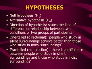
Null hypothesis testing • Difficult to evaluate specific expectations using classical null hypothesis testing: • Not always interested in null hypothesis • ‘accepting’ alternative hypothesis no answer • No direct relation • Visual inspection • Contradictory results
Null hypothesis testing • Theory • Expectations • Testing: • H0: nothing is going on vs. • H1: something is going on, but we do not know what… =catch-all hypothesis
Evaluating Informative Hypotheses • Theory • Expectations • Evaluating informative hypotheses: - Ha: theory/expectation 1 vs. - Hb: theory/expectation 2 vs. - Hc: theory/expectation 3 etc. √
Informative Hypotheses Hypothesized order constraints between statistical parameters • Order constraints: < > • Statistical parameters: means, regression coefficients, etc.
Why??? • Direct support for your expectation • Gain in power • Van de Schoot & Strohmeier, (2011), Testing informative hypotheses in SEM Increases Power. IJBD vol. 35 no. 2 180-190 7
Bayes factors for informative hypo’s • As was shown by Klugkist et al. (2005, Psych.Met.,10, 477-493), the Bayes factor (BF) of HA versus Hunc can be written as • where fi can be interpreted as a measure for model fit and ci as a measure for model complexity of Ha.
Bayes factors for informative hypo’s • Model Complexity, ci : • Can be computed before observing any data. • Determining the number of restrictions imposed on the means • The more restriction, the lower ci
Bayes factors for informative hypo’s • Model fit, fi : • After observing some data, • It quantifies the amount of agreement of the sample means with the restrictions imposed
Bayes factors for informative hypo’s • Bayesian Evaluation of Informative Hypotheses in SEM using Mplus • Van de Schoot, Hoijtink, Hallquist, & Boelen (in press). Bayesian Evaluation of inequality-constrained Hypotheses in SEM Models using Mplus. Structural Equation Modeling • Van de Schoot, Verhoeven & Hoijtink (under review). Bayesian Evaluation of Informative Hypotheses in SEM using Mplus: A Black Bear story.
Data • (1) females with a high score on negative coping strategies (n = 1429), • (2) females with a low score on negative coping strategies (n = 1532), • (3) males with a high score on negative coping strategies (n = 1545), • (4) males with a low score on negative coping strategies (n = 1072),
Model 17
Expectations • “We expected that the relation between life events on Time 1 is a stronger predictor of depression on Time 2 for girls who have a negative coping strategy than for girls with a less negative coping strategy and that the same holds for boys. Moreover, we expected that this relation is stronger for girls with a negative coping style compared to boys with a negative coping style and that the same holds for girls with a less negative coping style compared to boys with a less negative copings style.”
Expectations • Hi1 : (β1 > β2) & (β3 > β4) • Hi2 : β1 > (β2, β3) > β4)
Model 20
Bayes Factor 21
Step-by-step • we need to obtain estimates for fi and ci • Step 1. The first step is to formulate an inequality constrained hypothesis • Step 2. The second step is to compute ci. For simple order restricted hypotheses this can be done by hand.
Step-by-step • Count the number of parameters in the inequality constrained hypothesis • in our example: 4 (β1 β2 β3 β4) • Order these parameters in all possible ways: • in our example there are 4! = 4x3x2x1= 24 different ways of ordering four parameters.
Step-by-step • Count the number of possible orderings that are in line with each of the informative hypotheses: • For Hi1 (β1 > β2) & (β3 > β4) that are 6 possibilities; • For Hi2β1 > (β2, β3) > β4) that are 2 possibilities;
Step-by-step • Divide the value obtained in step 3 by the value obtained in step 2: • ci1 = 6/24 = 0.25 • ci2 = 2/24 = 0.0833 • Note that Hi2 is the most specific hypothesis and receives the smallest value for complexity.
Step-by-step • Step 3. Run the model in Mplus:
Mplus syntax DATA: FILE = data.dat; VARIABLE: NAMES ARE lif1 depr1 depr2 groups; MISSING ARE ALL (-9999); KNOWNCLASS is g(group = 1 group = 2 group = 3 group = 4); CLASSES is g(4);
Mplus syntax ANALYSIS: TYPE is mixture; ESTIMATOR = Bayes; PROCESSOR= 32;
Mplus syntax MODEL: %overall% depr2 on lif1; depr2 on depr1; lif1 with depr1; [lif1 depr1 depr2]; lif1 depr1 depr2;
Mplus syntax !save the parameter estimates for each iteration: SAVEDATA: BPARAMETERS are c:/Bayesian_results.dat;
R syntax To install MplusAutomation: R: install.packages(c("MplusAutomation")) R: library(MplusAutomation) Specify directory: R: setwd("c:/mplus_output")
R syntax Locate output file of Mplus: R: btest <- getSavedata_Bparams("output.out") Compute f1: R: testBParamCompoundConstraint (btest, "( STDYX_.G.1...DEPR2.ON.LIF_1 > STDYX_.G.2...DEPR2.ON.LIF_1) & STDYX_.G.3...DEPR2.ON.LIF_1 > TDYX_.G.4...DEPR2.ON.LIF_1)")
R syntax Compute f2: R: testBParamCompoundConstraint(btest, "( STDYX_.G.1...DEPR2.ON.LIF_1 > STDYX_.G.2...DEPR2.ON.LIF_1) & (STDYX_.G.3...DEPR2.ON.LIF_1 > STDYX_.G.4...DEPR2.ON.LIF_1) & (STDYX_.G.1...DEPR2.ON.LIF_1 > STDYX_.G.3...DEPR2.ON.LIF_1) & STDYX_.G.2...DEPR2.ON.LIF_1 > STDYX_.G.4...DEPR2.ON.LIF_1)")
Results • fi1 = .7573 • ci1= 0.25 • fi2 = .5146 • ci2 = 0.0833
Results • BF1 vsunc= .7573 / .25 = 3.03 • BF2 vsunc= .5146 / .0833 = 6.18
Results • BF1 vsunc= .7573 / .25 = 3.03 • BF2 vsunc= .5146 / .0833 = 6.18 • BF 2 vs 1 = 6.18 / 3.03 = 2.04
Conclusions • Excellent tool to include prior knowledge if available • Direct support for you expectations! • Gain in power