Download

1 / 31
330 likes | 363 Views
This chapter explores simple neural networks for pattern classification, including architectures, training procedures, learning rules, and exercises. Topics include Hebb's Rule, Perceptrons, Adaline, Delta Rule, and Madaline.

E N D
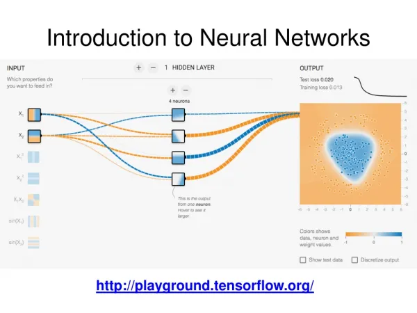
Introduction to Neural Networks John Paxton Montana State University Summer 2003
Chapter 2: Simple Neural Networks for Pattern Classification x0 1 w0 w0 is the bias f(yin) = 1 if yin >= 0 f(yin) = 0 otherwise ARCHITECTURE y w1 x1 wn xn
Representations • Binary: 0 no, 1 yes • Bipolar: -1 no, 0 unknown, 1 yes • Bipolar is superior
Interpreting the Weights • w0 = -1, w1 = 1, w2 = 1 • 0 = -1 + x1 + x2 or x2 = 1 – x1 YES x1 NO x2 decision boundary
Modelling a Simple Problem • Should I attend this lecture? • x1 = it’s hot • x2 = it’s raining x0 2.5 y -2 x1 1 x2
Linear Separability 1 0 1 1 0 1 0 0 1 0 1 0 AND OR XOR
Hebb’s Rule • 1949. Increase the weight between two neurons that are both “on”. • 1988. Increase the weight between two neurons that are both “off”. • wi(new) = wi(old) + xi*y
Algorithm 1. set wi = 0 for 0 <= i <= n 2. for each training vector 3. set xi = si for all input units 4. set y = t 5. wi(new) = wi(old) + xi*y
Result Interpretation • -2 + 2x1 + 2x2 = 0 OR • x2 = -x1 + 1 • This training procedure is order dependent and not guaranteed.
Pattern Recognition Exercise • #.# .#..#. #.##.# .#. “X” “O”
Pattern Recognition Exercise • Architecture? • Weights? • Are the original patterns classified correctly? • Are the original patterns with 1 piece of wrong data classified correctly? • Are the original patterns with 1 piece of missing data classified correctly?
Perceptrons (1958) • Very important early neural network • Guaranteed training procedure under certain circumstances x0 1 w0 y w1 x1 wn xn
Activation Function • f(yin) = 1 if yin > q f(yin) = 0 if -q <= yin <= q f(yin) = -1 otherwise • Graph interpretation 1 -1
Learning Rule • wi(new) = wi(old) + a*t*xi if error • a is the learning rate • Typically, 0 < a <= 1
Algorithm 1. set wi = 0 for 0 <= i <= n (can be random) 2. for each training exemplar do 3. xi = si 4. yin = S xi*wi 5. y = f(yin) 6. wi(new) = wi(old) + a*t*xi if error 7. if stopping condition not reached, go to 2
Example: AND concept • bipolar inputs • bipolar target • q = 0 • a = 1
Exercise • Continue the above example until the learning algorithm is finished.
Perceptron Learning Rule Convergence Theorem • If a weight vector exists that correctly classifies all of the training examples, then the perceptron learning rule will converge to some weight vector that gives the correct response for all training patterns. This will happen in a finite number of steps.
Exercise • Show perceptron weights for the 2-of-3 concept
Adaline (Widrow, Huff 1960) • Adaptive Linear Network • Learning rule minimizes the mean squared error • Learns on all examples, not just ones with errors
Architecture x0 1 w0 y w1 x1 wn xn
Training Algorithm 1. set wi (small random values typical) 2. set a (0.1 typical) 3. for each training exemplar do 4. xi = si 5. yin = S xi*wi 6. wi(new) = wi(old) + a*(t – yin)*xi 7. go to 3 if largest weight change big enough
Activation Function • f(yin) = 1 if yin >= 0 • f(yin) = -1 otherwise
Delta Rule • squared error E = (t – yin)2 • minimize error E’ = -2(t – yin)xi = a(t – yin)xi
Example: AND concept • bipolar inputs • bipolar targets • w0 = -0.5, w1 = 0.5, w2 = 0.5 • minimizes E
Exercise • Demonstrate that you understand the Adaline training procedure.
Madaline • Many adaptive linear neurons 1 1 y x1 z1 xm zk
Madaline • MRI (1960) – only learns weights from input layer to hidden layer • MRII (1987) – learns all weights