Download
1 / 30
340 likes | 421 Views
Introduction to Neural Networks. Marina Brozovi ć. References: talks by Matyas Bartok; Imperial College Goeffrey Hinton, U of Toronto Diana Spears, U of Wayoming

E N D
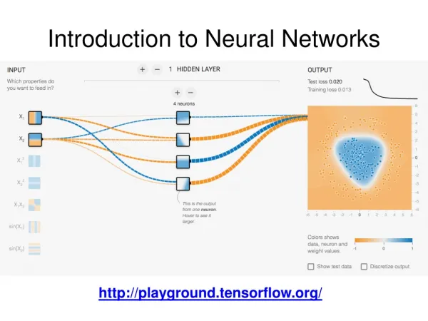
Introduction to Neural Networks Marina Brozović References: talks by Matyas Bartok; Imperial College Goeffrey Hinton, U of Toronto Diana Spears, U of Wayoming Nadia Bolshakova. Trinity College Dublin
Neural Network Characteristics • Basis: • a crude low-level model of biological neural systems • Powerful: • capable of modeling very complex functions/relationships • Ease of Use: • learns the structure for you, i.e. avoids need for formulating rules • user must deal with type of network, complexity, learning algorithms & inputs to use
History of Neural Networks • Attempts to mimic the human brain date back to work in the 1930s, 1940s, & 1950s by Alan Turing, Warren McCullough, Walter Pitts, Donald Hebb and James von Neumann • 1957 Rosenblatt at Cornell developed Perceptron, a hardware neural net for character recognition • 1959 Widrow and Hoff at Stanford developed NN for adaptive control of noise on telephone lines
History of Neural Networks, cont. • 1960s & 1970s period hindered by inflated claims and criticisms of the early work • 1982 Hopfield, a Caltech physicist, mathematically tied together many of the ideas from previous research. • Since then, growth has exploded. Thousands of research papers and commercial software applications
Types of Problems • Classification: determine to which of a discrete number of classes a given input case belongs • equivalent to logistic regression • Regression: predict the value of a (usually) continuous variable • equivalent to least-squares linear regression • Times series - you wish to predict the value of variables from earlier values of the same or other variables
Basic Artificial Model • Consists of simple processing elements called neurons, units or nodes • Each neuron is connected to other nodes with an associated weight(strength) which typically multiplies the signal transmitted • Each neuron has a single threshold value • Weighted sum of all the inputs coming into the neuron is formed and the threshold is subtracted from this value = activation • Activation signal is passed through an activation function(a.k.a. transfer function) to produce the output of the neuron
Real vs artificial neurons dendrites axon cell synapse dendrites x1 w1 Threshold units o xn wn
Processing at a Node weight 1 Activation Function Output weight 2 1.0 Sum 0.5 weight 3 Sum weight 4
Transfer Functions Determines how neuron scales its response to incoming signals Hard-Limit Sigmoid Radial Basis Threshold Logic
Purpose of the Activation Function g • We want the unit to be “active” (near +1) when the “right” inputs are given • We want the unit to be “inactive” (near 0) when the “wrong” inputs are given. • It’s preferable for g to be nonlinear. Otherwise, the entire neural network collapses into a simple linear function.
Feedforward networks These compute a series of transformations Typically, the first layer is the input and the last layer is the output. Recurrent networks These have directed cycles in their connection graph. They can have complicated dynamics. More biologically realistic. Types of connectivity output units hidden units input units
Types of Training • Supervised: most common • user provides data set of inputs with corresponding output(s) • training is performed until the network learns to associate each input vector to its respective and desired output vector • the relationship learned can then be applied to new data with unknown output(s) • Unsupervised • only input vectors are supplied • network learns some internal features of the whole set of input vectors presented to it • Reinforcement learning • combination of the above two paradigms
Math Review Dot product: Partial derivative: Hold all vj where j = i fixed, then take the derivative. Gradient: The gradient points in the direction of steepest ascent of the function f.
oi wji xj Perceptron Training • Can be trained on a set of examples using a special learning rule (process) • Weights are changed in proportion to the difference (error) between target output and perceptron solution for each example (p). • Minimize summed square error function: E = 1/2 ∑p∑i(oi(p) - ti(p))2 with respect to the weights.
Perceptron Training • Error minimized by finding set of weights that correspond to global minimum. • Done with gradient descent method – (weights incrementally updated in proportion to δE/δwij) • Updating reads: wji(t + 1) = wji(t) – Δwji, where Δwji = -ηδE/δwji. • Aim is to produce a true mapping for all patterns
Why does the method work? • For perceptrons, the error surface in weight space has a single global minimum and no local minima. Gradient descent is guaranteed to find the global minimum, provided the learning rate is not so big that that you overshoot it.
Math Review Chain rule for derivatives: (the chain rule can also be applied if these are partial derivatives)
“neti” Sigmoid unit for g x1 w1 oi xn wn Learning Rule for Sigmoid unit
Problems x1 • Perceptrons can only perform accurately with linearly separable classes (linear hyperplane can place one class of objects on one side of plane and other class on other) • ANN research put on hold for 20yrs. • Solution: additional (hidden) layers of neurons, MLP architecture • Able to solve non-linear classification problems x2 x1 x2
output units hidden units input units Hidden Units • Layer of nodes between input and output nodes • Allow a network to learn non-linear functions • Allow the net to represent combinations of the input features • With two possibly very large hidden layers, it is possible to implement any function
Common Questions About Neural Networks • How many hidden layers should I use? • As problem complexity increases, number of hidden layers should also increase • Start with none. Add hidden layers one at a time if training or testing results do not achieve target accuracy levels
oi xj yk Learning the Weights Between Hidden and Output Recall the perceptron learning rule; Error at output node i Weight update:
Error Back-Propagation to LearnWeights Between Input and Hidden • Key idea: each hidden node is responsible for some fraction of the error in each of the output nodes. This fraction equals the strength of the connection (weight) between the hidden node and the output node. where is the error at output node i. Errj
Learning Between Input and Hidden The update rule is now the standard, with notation adjusted to suit the situation: oi xj yk
Summary of BP learning algorithm • Initialize wji and wkj with random values. • Repeat until wji and wkj have converged or the desired performance level is reached: • Pick pattern p from training set. • Present input and calculate the output. • Update weights according to: wji(t + 1) = wji(t) – Δwji wkj(t + 1) = wkj(t) – Δwkj where Δw = -ηδE/δw. (…etc…for extra hidden layers).
Does BP always work on MLP? • Training of MLP using BP can be thought of as a walk in weight space along an energy surface, trying to find global minimum and avoiding local minima • Unlike for Perceptron, there is no guarantee that global minimum will be reached, but most cases energy landscape is smooth
Other Learning Algorithms • Back Propagation (first derivative): most popular • modifications exist: momentum propagation, resilient backprop • Others (some use second derivative of the error surface): Conjugate gradient descent, Levenberg-Marquardt, Quasi-Newton algorithm…
Future reading/exploring… • The GURU of neural nets: Geoffrey Hinton • www.cs.toronto.edu/~hinton/ (lookup his excellent NN lecture notes) • Matlab has a very good NN toolbox • Classical textbook : Christopher M Bishop, “Neural Networks for Pattern Recognition” • Other useful mathematical algorithms: Kalman Filters