Download
1 / 24
270 likes | 511 Views
Introduction to Neural Networks. John Paxton Montana State University Summer 2003. Chapter 6: Backpropagation. 1986 Rumelhart, Hinton, Williams Gradient descent method that minimizes the total squared error of the output. Applicable to multilayer, feedforward, supervised neural networks.

E N D
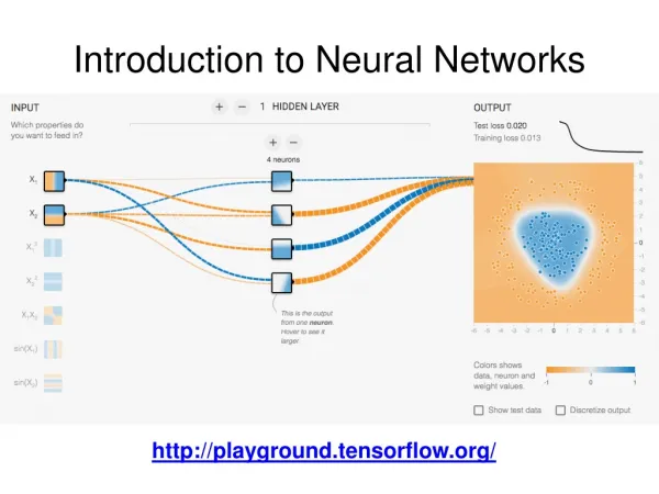
Introduction to Neural Networks John Paxton Montana State University Summer 2003
Chapter 6: Backpropagation • 1986 Rumelhart, Hinton, Williams • Gradient descent method that minimizes the total squared error of the output. • Applicable to multilayer, feedforward, supervised neural networks. • Revitalizes interest in neural networks!
Backpropagation • Appropriate for any domain where inputs must be mapped onto outputs. • 1 hidden layer is sufficient to learn any continuous mapping to any arbitrary accuracy! • Memorization versus generalization tradeoff.
Architecture • input layer, hidden layer, output layer 1 1 y1 x1 z1 ym xn zp wpm vnp
General Process • Feedforward the input signals. • Backpropagate the error. • Adjust the weights.
Activation Function Characteristics • Continuous. • Differentiable. • Monotonically nondecreasing. • Easy to compute. • Saturates (reaches limits).
Activation Functions • Binary Sigmoid f(x) = 1 / [ 1 + e-x ] f’(x) = f(x)[1 – f(x)] • Bipolar Sigmoid f(x) = -1 + 2 / [1 + e-x] f’(x) = 0.5 * [1 + f(x)] * [1 – f(x) ]
Training Algorithm 1. initialize weights to small random values, for example [-0.5 .. 0.5] 2. while stopping condition is false do steps 3 – 8 3. for each training pair do steps 4-8
Training Algorithm 4. zin.j = S (xi * vij) zj = f(zin.j) 5. yin.j = S (zi * wij) yj = f(yin.j) 6. error(yj) = (tj – yj) * f’(yin.j) tj is the target value 7. error(zk) = [ S error(yj) * wkj ] * f’(zin.k)
Training Algorithm 8. wkj(new) = wkj(old) + a*error(yj)*zk vkj(new) = vkj(old) + a*error(zj))*xk a is the learning rate An epoch is one cycle through the training vectors.
Choices • Initial Weights • random [-0.5 .. 0.5], don’t want the derivative to be 0 • Nguyen-Widrowb = 0.7 * p(1/n) n = number of input units p = number of hidden units vij = b * vij(random) / || vj(random) ||
Choices • Stopping Condition (avoid overtraining!) • Set aside some of the training pairs as a validations set. • Stop training when the error on the validation set stops decreasing.
Choices • Number of Training Pairs • total number of weights / desired average error on test set • where the average error on the training pairs is half of the above desired average
Choices • Data Representation • Bipolar is better than binary because 0 units don’t learn. • Discrete values: red, green, blue? • Continuous values: [15.0 .. 35.0]? • Number of Hidden Layers • 1 is sufficient • Sometimes, multiple layers might speed up the learning
Example • XOR. • Bipolar data representation. • Bipolar sigmoid activation function. • a = 1 • 3 input units, 5 hidden units,1 output unit • Initial Weights are all 0. • Training example (1 -1). Target: 1.
Example 4. z1 = f(1*0 + 1*0+ -1*0) = 0.5 z2 = z3 = z4 = 0.5 5. y1 = f(1*0 + 0.5*0 + 0.5*0 + 0.5*0 + 0.5*0) = 0.5 6. error(y1) = (1 – 0.5) * [0.5 * (1 + 0) * (1 – 0)] = 0.25 7. error(z1) = 0 * f’(zin.1) = 0 = error(z2) = error(z3) = error(z4)
Example 8. w01(new) = w01(old) + a*error(y1)*z0 = 0 + 1 * 0.25 * 1 = 0.25 v21(new) = v21(old) + a*error(z1)*x2 = 0 + 1 * 0 * -1 = 0.
Exercise • Draw the updated neural network. • Present the example 1 -1 as an example to classify. How is it classified now? • If learning were to occur, how would the network weights change this time?
XOR Experiments • Binary Activation/Binary Representation: 3000 epochs. • Bipolar Activation/Bipolar Representation: 400 epochs. • Bipolar Activation/Modified Bipolar Representation [-0.8 .. 0.8]: 265 epochs. • Above experiment with Nguyen-Widrow weight initialization: 125 epochs.
Variations • MomentumD wjk(t+1) = a * error(yj) * zk + m * D wjk(t)D vij(t+1) = similar • m is [0.0 .. 1.0] • The previous experiment takes 38 epochs.
Variations • Batch update the weights to smooth the changes. • Adapt the learning rate. For example, in the delta-bar-delta procedure each weight has its own learning rate that varies over time. • 2 consecutive weight increases or decreases will increase the learning rate.
Variations • Alternate Activation Functions • Strictly Local Backpropagation • makes the algorithm more biologically plausible by making all computations local • cortical units sum their inputs • synaptic units apply an activation function • thalamic units compute errors • equivalent to standard backpropagation
Variations • Strictly Local Backpropagationinput cortical layer -> input synaptic layer ->hidden cortical layer -> hidden synaptic layer ->output cortical layer-> output synaptic layer-> output thalamic layer • Number of Hidden Layers
Hecht-Neilsen Theorem Given any continuous function f: In -> Rm where I is [0, 1], f can be represented exactly by a feedforward network having n input units, 2n + 1 hidden units, and m output units.