Download
1 / 15
150 likes | 296 Views
Inference for distributions: - Comparing two means. Comparing two means Two-sample z distribution Two independent samples t -distribution Two sample t -test Two-sample t -confidence interval Robustness Details of the two sample t procedures. Two-sample z distribution.

E N D
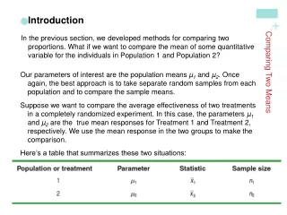
Comparing two means • Two-sample z distribution • Two independent samples t-distribution • Two sample t-test • Two-sample t-confidence interval • Robustness • Details of the two sample t procedures
Two-sample z distribution We have two independent SRSs (simple random samples) coming maybe from two distinct populations with (μ1,σ1) and (μ2, σ2). We use 1 and 2 to estimate the unknown μ1 and μ2. When both populations are normal, the sampling distribution of ( 1−2) is also normal, with standard deviation : Then the two-sample z statistic has the standard normal N(0, 1) sampling distribution.
Two independent samples t distribution We have two independent SRSs (simple random samples) coming maybe from two distinct populations with (μ1,σ1) and ((μ2, σ2) unknown. Use the sample means and sample s.d.s to estimate these unknown parameters. To compare the means, both populations should be normally distributed. However, in practice, it is enough that the two distributions have similar shapes and that the sample data contain no strong outliers.
The two-sample t statistic follows approximately the t distribution with a standard error SE (spread) reflecting variation from both samples: Conservatively, the degrees of freedom (df) is equal to the smallest of (n1 − 1, n2 − 1). df μ1 - μ2
Two-sample t-test The null hypothesis is that both population means μ1 and μ2 are equal, thus their difference is equal to zero. H0: μ1 = μ2 <=> μ1−μ2 = 0 with either a one-sided or a two-sided alternative hypothesis. We find how many standard errors (SE) away from (μ1−μ2) is ( 1−2) by standardizing: Because in a two-sample test H0assumes (μ1−μ2) = 0, we simply use With df = smallest(n1 − 1, n2 − 1)
Does smoking damage the lungs of children exposed to parental smoking? Forced vital capacity (FVC) is the volume (in milliliters) of air that an individual can exhale in 6 seconds. FVC was obtained for a sample of children not exposed to parental smoking and a group of children exposed to parental smoking. We want to know whether parental smoking decreases children’s lung capacity as measured by the FVC test. Is the mean FVC lower in the population of children exposed to parental smoking?
H0: μsmoke = μno <=> (μsmoke− μno) = 0 Ha:μ smoke < μno <=> (μsmoke− μno) < 0 (one sided) The difference in sample averages follows approximately the t distribution with 29 df: We calculate the t statistic: In table 3, for df 29 we find:|t| > 3.659 => p < 0.0005 (one sided) It’s a very significant difference, we reject H0. Lung capacity is significantly impaired in children of smoking parents.
C −t* t* Two sample t-confidence interval Because we have two independent samples we use the difference between both sample averages ( 1 −2) to estimate (μ1−μ 2). Practical use of t: t* • C is the area between −t* and t*. • We find t* in the line of Table 3 for df = smallest (n1−1; n2−1) and the column for confidence level C. • The margin of error MOE is:
Example: Can directed reading activities in the classroom help improve reading ability? A class of 21 third-graders participates in these activities for 8 weeks while a control classroom of 23 third-graders follows the same curriculum without the activities. After 8 weeks, all children take a reading test (scores in table). 95% confidence interval for (µ1 − µ2), with df = 20 conservatively t* = 2.086: With 95% confidence, (µ1 − µ2), falls within 9.96 ± 8.99 or 1.0 to 18.9.
Robustness “The two-sample t procedures are more robust than the one-sample t methods. When the sizes of the two samples are equal and the distributions of the two populations being compared have similar shapes, probability values from the t table are quite accurate for a broad range of distributions when the sample sizes are as small as n1 = n2 = 5” When planning a two-sample study, choose equal sample sizes if you can. As a guideline, a combined sample size (n1 + n2) of 40 or more will allow you to work even with the most skewed distributions. For very small samples though, make sure the data is very close to normal – no outliers, no skewness…
Details of the two sample t procedures The true value of the degrees of freedom for a two-sample t-distribution is quite lengthy to calculate. That’s why we use an approximate value, df = smallest(n1 − 1, n2 − 1), which errs on the conservative side (often smaller than the exact). Computer software, though, gives the exact degrees of freedom—or the rounded value—for your sample data.
Pooled two-sample procedures There are two versions of the two-sample t-test: one assuming equal variance (“pooled 2-sample test”)and one not assuming equal variance (“unequal” variance, as we have studied)for the two populations. They have slightly different formulas and degrees of freedom. The pooled (equal variance) two-sample t-test was often used before computers because it has exactly the t distribution for degrees of freedom n1 + n2− 2. However, the assumption of equal variance is hard to check, and thus the unequal variance test is safer. Two normally distributed populations with unequal variances
When both populations have the same standard deviation, the pooled estimator of σ2 is: The sampling distribution for (x1 − x2) has exactly the t distribution with (n1 + n2 − 2) degrees of freedom. A level C confidence interval for µ1 − µ2 is (with area C between −t* and t*) To test the hypothesis H0: µ1 = µ2against a one-sided or a two-sided alternative, compute the pooled two-sample t statistic for the t(n1 + n2 − 2) distribution.
For next time: Be sure to carefully read through sections 6.1 and 6.2 Then work on: #6.1, 6.4, 6.5, 6.10, 6.12