Download
1 / 11
110 likes | 232 Views
Material from Hoskins et al. 1985. Cyclonic PV anomaly.

E N D
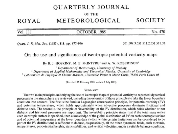
Cyclonic PV anomaly • Figure I5. Circularly symmetric flows induced by simple, isptated, IPV anomalies (whose locations are shown stippled) as described in the text. The basic static stability Nand therefore P (defined in (34)) was uniform in the tropospheric region and six times larger in the stratospheric region. The vertica1 coordinate z is nearly the same as physical height but is defined exactly in (35), g/Oo being taken to be (1/30)ms-2K-'. The reference tropospheric 'height' z was 10 km and the total domain 'height' 16.67 km: f was taken to be 10-4s-'. The IPV anomaly was defined by takin the tropopause potential temperature to vary in the manner &4{cos(nF/ro) + 1) may be compared with a potential temperature increase of 30 K over the depth of the reference troposphere. The parameter ro was taken to be 1667 km. The undisturbed 0 distribution was imposed as a boundary condition at i = 5000 km, and the solutions obtained had only a weak dependence of Cb(0) upon 0 as well as a far-field stratification approximating the reference stratification (16). (In terms of our definitions, the IPV anomaly in the stippled regions must therefore strictly speaking be considered to be embedded in a suitable 'surround' of much weaker anomalies, as noted below (17b).) Only the region r < 25OO km is shown here, and the tick marks below the axes are drawn every 833 km. The thick line represents the tropopause and the two sets of thin lines the isentropes every 5 K and the transverse velocity every 3 m s-'. The zero isotach on the axis of symmetry is omitted. In (a) the sense of the azimuthal wind is cyclonic and in (b) it is anticyclonic, in both cases the maximum contour value being 21 m s-'. The surface pressure anomaly is -41 mb in (a) and + 13 mb in (b) and the relative vorticity extrema (located at the tropopause) are 1.7fin (a) and -0.6fin (b). The maximum surface winds are 15 m s-' and 6 ms-' respectively. For more details of the method of computation, see Thorpe (1985).
Anticyclonic PV anomaly • Figure IS. Circularly symmetric flows induced by simple, isptated, IPV anomalies (whose locations are shown stippled) as described in the text. The basic static stability Nand therefore P (defined in (34)) was uniform in the tropospheric region and six times larger in the stratospheric region. The vertica1 coordinate z is nearly the same as physical height but is defined exactly in (35), g/Oo being taken to be (1/30)ms-2K-'. The reference tropospheric 'height' z was 10 km and the total domain 'height' 16.67 km: f was taken to be 10-4s-'. The IPV anomaly was defined by takin the tropopause potential temperature to vary in the manner &4{cos(nF/ro) + 1) may be compared with a potential temperature increase of 30 K over the depth of the reference troposphere. The parameter ro was taken to be 1667 km. The undisturbed 0 distribution was imposed as a boundary condition at i = 5000 km, and the solutions obtained had only a weak dependence of Cb(0) upon 0 as well as a far-field stratification approximating the reference stratification (16). (In terms of our definitions, the IPV anomaly in the stippled regions must therefore strictly speaking be considered to be embedded in a suitable 'surround' of much weaker anomalies, as noted below (17b).) Only the region r < 25OO km is shown here, and the tick marks below the axes are drawn every 833 km. The thick line represents the tropopause and the two sets of thin lines the isentropes every 5 K and the transverse velocity every 3 m s-'. The zero isotach on the axis of symmetry is omitted. In (a) the sense of the azimuthal wind is cyclonic and in (b) it is anticyclonic, in both cases the maximum contour value being 21 m s-'. The surface pressure anomaly is -41 mb in (a) and + 13 mb in (b) and the relative vorticity extrema (located at the tropopause) are 1.7fin (a) and -0.6fin (b). The maximum surface winds are 15 m s-' and 6 ms-' respectively. For more details of the method of computation, see Thorpe (1985).for T < ro, where F = r(Xoc/f)' 9 2. Here the amplitude A was taken to be -24 K in (a) and +24 K in (b) which “the anomaly in P appears partly as absolute vorticity and partly as static stability. The proportions in which this partitioning occurs can be shown to depend on the shape of the anomaly, a broad, shallow anomaly tending to realize P more as static stability and a tall one more as absolute vorticity”
Large-scale Cyclonic PV feature: influence all the way to the surface
Synoptic scale cyclonic PV feature at upper levels (doesn’t reach surface)
Anticyclone near tropopause As far as gross features are concerned, everything is the opposite way round from Figs. 8-10. The tropopause is high, the isentropes in the troposphere bow downwards, and those in the stratosphere bow upwards. The very low potential vorticity just under the tropopause, less than 0.5 PV units, is particularly striking. Once again we shall see that this structure is just that expected theoretically for the fields induced by an isolated, upper air IPV anomaly of the appropriate sign.
Surface theta “is” PV a warm surface potential temperature anomaly is equivalent to a cyclonic IPV anomaly concentrated at the surface. As statement (i) of section 3 predicts, it induces a cyclonic vortex (Fig. 16(a)). A cold surface anomaly induces an anticyclonic vortex (Fig. 16(b)).