Download

1 / 35
350 likes | 456 Views
Theories and Methods of the Business Cycle. Part 1: Dynamic Stochastic General Equilibrium Models IV. Can RBC be saved? Jean-Olivier HAIRAULT , Professeur à Paris I Panthéon-Sorbonne et à l’Ecole d’Economie de Paris (EEP). IV. 1. Extending the RBC approach.

E N D
Theories and Methods of the Business Cycle. Part 1: Dynamic Stochastic General Equilibrium Models IV. Can RBC be saved? Jean-Olivier HAIRAULT, Professeur à Paris I Panthéon-Sorbonne et à l’Ecole d’Economie de Paris (EEP)
IV. 1. Extending the RBC approach • Two kinds of extensions: solving empirical puzzles and investigating other issues. • Some criticisms have been adressed into the RBC theory, ie. models where productivity shocks are the main perturbation of optimal fluctuations. • The canonical model has been extended to international fluctuations and to the study of particular historical episodes like the 1930’s crisis.
IV. 2. Public spending shocks w E’ E E’’ Ns, Nd
IV. 2. Public spending shocks • Government shocks have wealth effects which alters labor supply. The correlation between wages and hours is then negative in case of government shocks. • Taking into account both shocks leads to decrease this correlation. E’’ E E’
IV. 2. Public spending shocks • Business cycles properties with public expenditures shocks • From kprdea2.m to kprdea2G.m • The correlation between hours and wages is decreased but remains too high. Public expenditures shocks have a weaker impact on aggregates than technology shocks. • Artificially decreasing the volatility of the technology shocks could lead to a negative correlation.
IV. 2. Public spending shocks • Only Technology ShocksN Y C I P • standard deviation 0.0081 0.0142 0.0050 0.0523 0.0066 • relative st. dev. 0.5667 1.0000 0.3480 3.6733 0.4655 • Correlation 0.9745 1.0000 0.8910 0.9864 0.9623 • serial corr. 0.6750 0.6924 0.7972 0.6770 0.6924 • correlation N-W 0.8770 • +public spending shocks • standard deviation 0.0069 0.0134 0.0062 0.0486 0.0074 • relative st. dev. 0.5187 1.0000 0.4634 3.6346 0.5519 • Correlation 0.9290 1.0000 0.8569 0.9816 0.9380 • serial correlation 0.6808 0.6920 0.7715 0.6798 0.6920 • correlation N-W 0.7441
IV. 3.Back to the Lucas critique • RBC methodology allows us to take into account all the implications of a change in public policy or in the environment of private agents. • The dynamics derive from the interaction between the environment (shocks, public policies) and fundamentals (Technology, preferences). • Which public spending rule does better stabilize the economy? • Volatility ? Which volatility? • Welfare? What are the market failures in our economy? • What are the size of business cycle costs? More on this issue in course 6.
IV. 4. The indivisible labor hypothesis • Eta=1 N Y C I P • standard deviation 0.0081 0.0142 0.0050 0.0523 0.0066 • relative st. dev. 0.5667 1.0000 0.3480 3.6733 0.4655 • Correlation 0.9745 1.0000 0.8910 0.9864 0.9623 • serial corr. 0.6750 0.6924 0.7972 0.6770 0.6924 • correlation N-W 0.8770 • Infinite elasticity • standard deviation 0.0124 0.0170 0.0057 0.0638 0.0057 • relative st. Dev. 0.7270 1.0000 0.3329 3.7442 0.3329 • Correlation 0.9750 1.0000 0.8759 0.9865 0.8759 • serial correlation 0.6706 0.6883 0.8034 0.6727 0.6883 • correlation N-W 0.7472
IV. 6. Labor Hoarding • Taking into account the quality or intensity of worked hours • labor intensity increases (decreases) in expansions (contractions). • Firms prefer to adjust labor intensity rather employment. Individual hours are assumed to be indivisible and employment are submitted to adjustment costs. Employment gets predetermined. • Productivity cycle: labor productivity measured as output/employment leads employment in the data. • Correlation lagged and contemporanous productivity-employment: .11 0.37 0.47 0.47 0.34
IV. 6. Labor Hoarding • Y = A F(K, X(eH)) • The Solow Residual is no longer a pure measure of technology: variations of e must be eliminated. • Naive Solow residual overestimates the standart deviation of the technology innovation by 35%, as estimated by Burnside, Christiano and Rebelo. • Technology shocks are not volatile enough to replicate the variance of output. Only 58%. • Adding another real shock: public spending.
IV. 7. International Business Cycles • Backus, Kehoe and Kydland [1992], Journal of Political Economy, Baxter [1995], Hanbook of International Economics • More failures than in closed economies due to capital international mobility and portfolio diversification…but at the origin of the new open economy macroeconomics, Obstfeld and Rogoff [1995]. I will present some international RBC models in the open macroeconomics course…
IV. 7. International Business Cycles • After a technology shock abroad, aggregates increase as in the closed RBC economy. • As the capital return is higher abroad, domestic households invest abroad: the capital stock decreases in the domestic country, and so the labor demand decreases too. This explains why the model predicts a negative correlation between production factors across countries. • Output across countries is then less correlated in the model than in the data. • As there is perfect risk-sharing (complete markets), the marginal utility of consumption is equalized across countries: the wealth distribution does not vary over the business cycle. In case of positive shock abroad, the domestic receives a payment provided by a state-contingent security. • Consumption across countries is then more correlated in the model than in the data.
IV. 8. The Great Depression • Special issue of the Review of Economic Dynamics in 2002 investigating the 1930’s crisis in the main developed countries using the RBC model • P. Beaudry and F. Portier [2002], RED, The French Depression in the 1930’s


![[Notes 12]](https://cdn0.slideserve.com/443045/notes-12-dt.jpg)