Download
1 / 26
270 likes | 383 Views
Statistic Process Control. Week 3 Ananda Sabil Hussein, SE, MCom. Latar Belakang. Pertengahan tahun 80 an pangsa pasar pager Motorola di rebut oleh produk-produk Jepang seperti halnya NEC, TOSHIBA dan Hitachi.

E N D
Statistic Process Control Week 3 Ananda Sabil Hussein, SE, MCom
Latar Belakang • Pertengahan tahun 80 an pangsa pasar pager Motorola di rebut oleh produk-produk Jepang seperti halnya NEC, TOSHIBA dan Hitachi. • Motorola melakukan perubahan radikal dengan memperbaiki mutu, pengembangan produk dan penurunan biaya yang berbasis statistik
Statistical Process Control • Teknik statistik yang secara luas digunakan untuk memastikan bahwa proses yang sedang berjalan telah memenuhi standar.
Produce Good Start Provide Service No Assign. Take Sample Causes? Yes Inspect Sample Stop Process Create Find Out Why Control Chart
Variasi Alami dan Khusus • Variasi alami adalah sumber-sumber variasi dalam proses yang secara statistik berada dalam batas kendali • Variasi Khusus/dapat dihilangkan yaitu variasi yang muncul disebabkan karena peralatan yang tidak sesuai, karyawan yang lelah atau kurang terlatih serta bahan baku baru.
17 = UCL 16 = Mean 15 = LCL | | | | | | | | | | | | 1 2 3 4 5 6 7 8 9 10 11 12 Sample number
Konsep Rata-rata dan Jarak Rata-rata
Menentukan Batas Diagram Rata-rata • Batas Kendali Atas (UCL) = • Batas Kendali Bawah (LCL) = • = rata-rata dari sampel = = Standar deviasi = 2 (95.5%) 3(99.7%) = Standar deviasi rata-rata sampel
Cara Lain Batas Kendali Atas = Batas Kendali Bawah Dimana : = rentangan rata-rata sampel = Nilai batas kendali = rata-rata dari sampel rata-rata
(a) These sampling distributions result in the charts below (Sampling mean is shifting upward but range is consistent) UCL (x-chart detects shift in central tendency) x-chart LCL UCL (R-chart does not detect change in mean) R-chart LCL Bagan Rata-rata
(b) These sampling distributions result in the charts below (Sampling mean is constant but dispersion is increasing) UCL (x-chart does not detect the increase in dispersion) x-chart LCL UCL (R-chart detects increase in dispersion) R-chart LCL Bagan Jarak Figure S6.5
Bagan Kendali Atribut • Mengukur persentase penolakan dalam sebuah sampel, bagan-p • Menghitung jumlah penolakan, bagan-c
Control Charts for Attributes • For variables that are categorical • Good/bad, yes/no, acceptable/unacceptable • Measurement is typically counting defectives • Charts may measure • Percent defective (p-chart) • Number of defects (c-chart)
p(1 - p) n sp = UCLp = p + zsp ^ ^ LCLp = p - zsp ^ where p = mean fraction defective in the sample z = number of standard deviations sp = standard deviation of the sampling distribution n = sample size ^ Control Limits for p-Charts Population will be a binomial distribution, but applying the Central Limit Theorem allows us to assume a normal distribution for the sample statistics
Ditanyakan : Batas kendali proses 9 boks yang mencakup 99.7% • Jawab : = 16 + 3 UCLx = LCLx = = 16 - 3
Process average x = 16.01 ounces Average range R = .25 Sample size n = 5 Setting Control Limits
Process average x = 16.01 ounces Average range R = .25 Sample size n = 5 UCLx = x + A2R = 16.01 + (.577)(.25) = 16.01 + .144 = 16.154 ounces From Table S6.1 Setting Control Limits
Process average x = 16.01 ounces Average range R = .25 Sample size n = 5 UCLx = x + A2R = 16.01 + (.577)(.25) = 16.01 + .144 = 16.154 ounces UCL = 16.154 Mean = 16.01 LCLx = x - A2R = 16.01 - .144 = 15.866 ounces LCL = 15.866 Setting Control Limits
Sample Number Fraction Sample Number Fraction Number of Errors Defective Number of Errors Defective 1 6 .06 11 6 .06 2 5 .05 12 1 .01 3 0 .00 13 8 .08 4 1 .01 14 7 .07 5 4 .04 15 5 .05 6 2 .02 16 4 .04 7 5 .05 17 11 .11 8 3 .03 18 3 .03 9 3 .03 19 0 .00 10 2 .02 20 4 .04 Total = 80 (.04)(1 - .04) 100 80 (100)(20) sp = = .02 p = = .04 ^ Contoh Soal
UCLp= 0.10 .11 – .10 – .09 – .08 – .07 – .06 – .05 – .04 – .03 – .02 – .01 – .00 – LCLp= 0.00 UCLp = p + zsp= .04 + 3(.02) = .10 ^ Fraction defective p = 0.04 LCLp = p - zsp = .04 - 3(.02) = 0 ^ | | | | | | | | | | 2 4 6 8 10 12 14 16 18 20 Sample number p-Chart for Data Entry
UCLp= 0.10 .11 – .10 – .09 – .08 – .07 – .06 – .05 – .04 – .03 – .02 – .01 – .00 – LCLp= 0.00 UCLp = p + zsp= .04 + 3(.02) = .10 ^ Fraction defective p = 0.04 LCLp = p - zsp = .04 - 3(.02) = 0 ^ | | | | | | | | | | 2 4 6 8 10 12 14 16 18 20 Sample number p-Chart for Data Entry Possible assignable causes present
UCLc = c + 3 c LCLc = c - 3 c where c = mean number defective in the sample Control Limits for c-Charts Population will be a Poisson distribution, but applying the Central Limit Theorem allows us to assume a normal distribution for the sample statistics
c = 54 complaints/9 days = 6 complaints/day UCLc = c + 3 c = 6 + 3 6 = 13.35 UCLc= 13.35 14 – 12 – 10 – 8 – 6 – 4 – 2 – 0 – Number defective LCLc = c - 3 c = 3 - 3 6 = 0 c = 6 LCLc= 0 | 1 | 2 | 3 | 4 | 5 | 6 | 7 | 8 | 9 Day c-Chart for Cab Company