Download

1 / 32
320 likes | 456 Views
The Investigation of Data Using Tables. The Investigation of Data Using Tables. Primary objective: to show how data is investigated in terms of tables using STATA Secondary objective: to demonstrate some of the features of STATA for general data management and analysis.

E N D
The Investigation of Data Using Tables Primary objective: to show how data is investigated in terms of tables using STATA Secondary objective: to demonstrate some of the features of STATA for general data management and analysis The definition and layout of a table The purpose of a table STATA commands for the examination of tabulated data Designing a table Preparing data for tabulation: coding, labeling, and screening Some statistical tests relating to tabulated data Some demonstrations of the application of tables Simple tables relating to purely categorical variables More complex tables of categorical variables and predicting probabilities Tabulation as a tool to summarize continuous data
The definition, and layout of a table A table is a matrix-like structure in which the elements characterize aspects of the categories of the table-defining variables Tables can be one, two, or three, or more dimensional - though tables with higher than three dimensions are hard to follow A one-way, or one dimensional table . table age ----------+----------- agecat | Freq. ----------+----------- 25-29 | 292 30-34 | 444 35-39 | 393 40-44 | 442 45-49 | 405 ----------+----------- A two-way, or two dimensional table . table age smoke ----------+----------------------------------------- | smokelev agecat | 0 per d. 1-24 per d. >=25 per d. ----------+----------------------------------------- 25-29 | 132 105 55 30-34 | 188 158 98 35-39 | 164 142 87 40-44 | 180 155 107 45-49 | 180 139 86 ----------+-----------------------------------------
A three-way table with marginal totals (row and column totals) . table age smoke, by(oc) row col ------------+------------------------------------------------------- ocuse and | smokelev agecat | 0 per d. 1-24 per d. >=25 per d. Total ------------+------------------------------------------------------- Non oc-user | 25-29 | 107 79 40 226 30-34 | 175 147 80 402 35-39 | 156 130 77 363 40-44 | 175 151 101 427 45-49 | 175 138 81 394 | Total | 788 645 379 1,812 ------------+------------------------------------------------------- Oc-user | 25-29 | 25 26 15 66 30-34 | 13 11 18 42 35-39 | 8 12 10 30 40-44 | 5 4 6 15 45-49 | 5 1 5 11 | Total | 56 54 54 164 ------------+-------------------------------------------------------
Attributes of a simple table categorical variables STATA table command smoking level categories . table age smoke ----------+----------------------------------------- | smokelev agecat | 0 per d. 1-24 per d. >=25 per d. ----------+----------------------------------------- 25-29 | 132 105 55 30-34 | 188 158 98 35-39 | 164 142 87 40-44 | 180 155 107 45-49 | 180 139 86 ----------+----------------------------------------- age categories number of study subjects in the specific categories from the study
The purpose of a table In regard to categorical variables the purpose of a table is: 1. to highlight trends in the cell counts by categories of the categorical variables 2. to highlight disproportionate presence of cell counts when considered in regard to the total number of individuals who could occupy the cells 3. to summarize categorized information, perhaps confirming balance, in a study, in regard to participant classes, or categories 4. to summarize outcomes, especially when outcomes are dichotomous, and gain a ‘quick’ appreciation of potentially significant study factors when preparing data for analysis and with respect to continuous data 5. to summarize continuous information possibly pointing to patterns of variability amongst classes of individuals
Trends in cell counts ... . table oc age, row col ------------+----------------------------------------- | agecat ocuse | 25-29 30-34 35-39 40-44 45-49 Total ------------+----------------------------------------- Non oc-user | 226 402 363 427 394 1,812 Oc-user | 66 42 30 15 11 164 | Total | 292 444 393 442 405 1,976 ------------+----------------------------------------- . table mi age, row col ----------+----------------------------------------- | agecat mi | 25-29 30-34 35-39 40-44 45-49 Total ----------+----------------------------------------- No MI | 286 423 356 371 306 1,742 MI | 6 21 37 71 99 234 | Total | 292 444 393 442 405 1,976 ----------+----------------------------------------- Note that for perceived trends to be significant the denominator must also be considered. It is actually a trend in proportions that we are looking for There is actually a Test for the Significance of trends in a table, see nptrend Trend direction Trend direction
Disproportionate presence of cell counts ... . table oc mi, row col ------------+-------------------- | mi ocuse | No MI MI Total ------------+-------------------- Non oc-user | 1,607 205 1,812 Oc-user | 135 29 164 | Total | 1,742 234 1,976 ------------+-------------------- Again, it is critical to ask disproportionate in regard to what … we again need a reference, or denominator Simply changing the command a little help us here . tabulate oc mi, col | mi ocuse | No MI MI | Total ------------+----------------------+---------- Non oc-user | 1607 205 | 1812 | 92.25 87.61 | 91.70 ------------+----------------------+---------- Oc-user | 135 29 | 164 | 7.75 12.39 | 8.30 ------------+----------------------+---------- Total | 1742 234 | 1976 | 100.00 100.00 | 100.00 Note the greater prevalence of mi amongst the oc users than the non-users
Confirming balance in a study in regard to participant classes, or categories ... . tabulate age smoke, row col | smokelev agecat | 0 per d 1-24 per >=25 per | Total -----------+---------------------------------+---------- 25-29 | 132 105 55 | 292 | 45.21 35.96 18.84 | 100.00 | 15.64 15.02 12.70 | 14.78 -----------+---------------------------------+---------- 30-34 | 188 158 98 | 444 | 42.34 35.59 22.07 | 100.00 | 22.27 22.60 22.63 | 22.47 -----------+---------------------------------+---------- 35-39 | 164 142 87 | 393 | 41.73 36.13 22.14 | 100.00 | 19.43 20.31 20.09 | 19.89 -----------+---------------------------------+---------- 40-44 | 180 155 107 | 442 | 40.72 35.07 24.21 | 100.00 | 21.33 22.17 24.71 | 22.37 -----------+---------------------------------+---------- 45-49 | 180 139 86 | 405 | 44.44 34.32 21.23 | 100.00 | 21.33 19.89 19.86 | 20.50 -----------+---------------------------------+---------- Total | 844 699 433 | 1976 | 42.71 35.37 21.91 | 100.00 | 100.00 100.00 100.00 | 100.00 Here we see the relative representation of every category by row variable and by column variable. It would not hurt to circle large percentages, and small percentages and explore their bases
. table oc, content(mean mi) ------------+----------- ocuse | mean(mi) ------------+----------- Non oc-user | .1131347 Oc-user | .1768293 ------------+----------- To summarize outcomes ... Here we see tabulations of the proportion of mi subjects in each of the age, smoking, and oc-use classes . table age smoke, contents(mean mi) by(oc) format(%7.4f) ------------+----------------------------------------- ocuse and | smokelev agecat | 0 per d. 1-24 per d. >=25 per d. ------------+----------------------------------------- Non oc-user | 25-29 | 0.0093 0.0000 0.0250 30-34 | 0.0000 0.0340 0.0875 35-39 | 0.0192 0.0846 0.2468 40-44 | 0.0571 0.1391 0.3366 45-49 | 0.1143 0.3043 0.3827 ------------+----------------------------------------- Oc-user | 25-29 | 0.0000 0.0385 0.2000 30-34 | 0.0000 0.0909 0.4444 35-39 | 0.0000 0.0833 0.3000 40-44 | 0.2000 0.0000 0.8333 45-49 | 0.6000 0.0000 0.6000 ------------+-----------------------------------------
To summarize continuous information ... In a study to explore the efficacy of a new drug, nifedipine, to alleviate chest pain in heart patients, subjects were treated with either propanolol or nifedipine and the pattern of their heart rate and blood pressure monitored at each stage of adjustment of either drug dosage. There were three stages of the study in addition to baseline (time zero). . table grp time, c(mean hr) format(%7.2f) ----------+------------------------------- | time grp | 0 1 2 3 ----------+------------------------------- N | 71.72 77.83 124.28 127.78 P | 76.81 79.69 97.81 112.75 ----------+------------------------------- Note the heart rate and systolic blood pressure patterns in time with the two drugs. Is this as useful as a graphical representation of the results? . table grp time, c(m sbp) format(%7.2f) ----------+------------------------------- | time grp | 0 1 2 3 ----------+------------------------------- N | 138.78 134.00 129.43 135.67 P | 144.91 136.55 136.57 140.86 ----------+-------------------------------
In this study, because all subjects did not proceed to each stage, we would be advised to explore the level of participation of each stage... . table grp time if sbp==. ----------+----------------------- | time grp | 0 1 2 3 ----------+----------------------- N | 9 9 11 12 P | 5 5 9 9 ----------+----------------------- Number of missing ‘sbp’ observations by group and study stage, amongst participants . table grp time if sbp~=. ----------+----------------------- | time grp | 0 1 2 3 ----------+----------------------- N | 9 9 7 6 P | 11 11 7 7 ----------+----------------------- Number of non-missing ‘sbp’ observations by group and study stage, amongst participants
An investigation into the missing values could also be advanced as follows: . generate miss=sbp==. . table time grp, by(miss) ----------+----------- miss and | grp time | N P ----------+----------- 0 | 0 | 9 11 1 | 9 11 2 | 7 7 3 | 6 7 ----------+----------- 1 | 0 | 9 5 1 | 9 5 2 | 11 9 3 | 12 9 ----------+----------- non-missing values missing values
STATA commands for the examination of tabulated data Tables are to categorical variables as summarization is to continuous variables … we use the STATA commands to investigate categorical variables in every sense. There are four STATA commands for the specific manipulation of tables …. tabulate …. table …. tabdisp …. tabstat [by varlist:] tabulate varname1 [varname2] [weight] [if exp] [in range] , summarize(varname3) [ [no]means [no]standard [no]freq [no]obs wrap nolabel missing ] table rowvar [colvar [supercolvar]] [weight] [if exp] [in range] [, contents(clist) by(superrow_varlist) cw row col scol format(%fmt) center left concise missing replace name(string) cellwidth(#) csepwidth(#) scsepwidth(#) stubwidth(#) ] tabdisp rowvar [colvar [supercolvar]] [if exp] [in range], cellvar(varnames) [ by(superrowvar(s)) format(%fmt) center left concise missing totals cellwidth(#) csepwidth(#) scsepwidth(#) stubwidth(#) ] tabstat varlist [if exp] [in range] [weight] [, statistics(statname [...]) by(varname) nototal missing nosep columns(variables|statistics) longstub labelwidth(#) format[(%fmt)] casewise save ]
USE tabulate (tab) to display simple summaries, relative cell counts, associative measures between row and column variables . tabulate case age [fweight=count], chi row col | age case | <= 29 >= 30 | Total -----------+----------------------+---------- Control | 8747 1498 | 10245 | 85.38 14.62 | 100.00 | 77.5268.68 | 76.09 -----------+----------------------+---------- Case | 2537 683 | 3220 | 78.79 21.21 | 100.00 | 22.4831.32 | 23.91 -----------+----------------------+---------- Total | 11284 2181 | 13465 | 83.80 16.20 | 100.00 | 100.00100.00 | 100.00 Pearson chi2(1) = 78.3698 Pr = 0.000
USE table to display statistics concerning variables in a table and to gain control of the table layout, for publication purposes . table time, c(mean hr mean sbp freq) format(%8.3f) by(grp) ----------+----------------------------------- grp and | time | mean(hr) mean(sbp) Freq. ----------+----------------------------------- N | 0 | 71.722 138.778 18 1 | 77.833 134.000 18 2 | 124.278 129.429 18 3 | 127.778 135.667 18 ----------+----------------------------------- P | 0 | 76.812 144.909 16 1 | 79.688 136.545 16 2 | 97.812 136.571 16 3 | 112.750 140.857 16 ----------+-----------------------------------
USE tabdisp to display your own calculations, and observations, in a table in which you do not want any special treatment of the numbers . tabdisp case age, cellvar(Chi) format(%7.2f) ----------+------------- | age case | <= 29 >= 30 ----------+------------- Control | 3.04 15.71 Case | 9.66 49.97 ----------+------------- categorical variables ‘structuring’ the table values of the variable ‘chi’ displayed using the indicated format
USE tabstat to display the (same comprehensive array of) statistics of (several) variables in a table and to gain control of the table layout, for publication purposes, when only one classifying (categorical) variable is considered . tabstat hr* sbp*, by(grp) stat(mean med max sd) format(%6.2f) long grp stats | hr1 hr2 hr3 sbp1 sbp2 sbp3 -------------+------------------------------------------------------------ N mean | 77.83 124.28 127.78 134.00 129.43 135.67 p50 | 71.00 115.00 120.00 134.00 128.00 129.00 max | 125.00 230.00 230.00 160.00 150.00 180.00 sd | 21.00 49.55 44.41 15.84 17.08 28.38 -------------+------------------------------------------------------------ P mean | 79.69 97.81 112.75 136.55 136.57 140.86 p50 | 76.50 82.00 110.00 134.00 130.00 150.00 max | 120.00 190.00 180.00 180.00 206.00 188.00 sd | 19.95 45.45 47.34 22.40 36.29 27.85 -------------+------------------------------------------------------------ Tot mean | 78.71 111.82 120.71 135.40 133.00 138.46 p50 | 74.50 97.00 120.00 134.00 130.00 140.00 max | 125.00 230.00 230.00 180.00 206.00 188.00 sd | 20.22 48.82 45.75 19.27 27.50 27.03 -------------+------------------------------------------------------------ Note the use of the ‘*’ wildcard to ensure that all variables whose names started with ‘hr’ and ‘sbp’ are included in the table
Designing a table • Use the following principles in designing a table • Tables should be wider than they are long • The row and column headings should clearly describe the specific classes • Arrange entries in the table so that trends and differences are clear • Only use super-rows and super-columns sparingly, and check with journals • Ensure that the summary attribute of a cell is presented in proportion to its • importance (e.g. means should be more evident than errors) • Don’t over-crowd tables, numbers should be specified to no greater • precision than can be justified • When creating a table in an exploratory fashion carefully articulate the • categories to be ‘cross tabulated’ and the nature of the summarization you • require (See also Woodward, pp 39 – 44)
Preparing data for tabulation: coding, labeling, and screening A study (Rosner chap. 10) elucidated the following relationship between breast cancer (cases) in women and age at birth of first child | age case | <= 29 >= 30 | Total -----------+----------------------+---------- Control | 8747 1498 | 10245 Case | 2537 683 | 3220 -----------+----------------------+---------- Total | 11284 2181 | 13465 A number of questions arise if we want to investigate this data: how do we select a set of variables to represent this information? how do we decide on a coding scheme for the variables? how do we ensure that we can recall the coding pattern (labeling)? how do we reproduce the above table? how can we establish whether age at first birth and breast cancer are related?
how do we select a set of variables to represent this information There are two categorical variables, case/control, and age (<=29/>=30) that can be used to specify each cell in the table. Additionally, we’ll need a variable to quantify the number of entries in each cell. The variables are then, for example case age count how do we decide on a coding scheme for the variables The general approach to coding dichotomous categorical variables is to set the state of interest to the value ‘1’, and the other state to the value ‘0’. Here since we are concerned with breast cancer as the ‘case’ state, we will code the variable case as ‘1’ for case, ‘0’ for control. Note that pneumonic matching is also very important. Similarly, our exposure is delaying first birth, so our state of interest is age>=30, so we will code age as ‘1’ for age >= 30, and ‘0’ otherwise.
We will code the variable count as given by cell occupancy in the table Summarizing: 1: breast cancer case case 0: non-breast cancer (i.e. control) 1: age>=30 at first birth age 0: age<=29 at first birth count cell frequency or occupancy Is ‘case’ actually a good name for the variable here?
Now we have the following table: . list age case count 1. 0 0 8747 2. 0 1 2537 3. 1 0 1498 4. 1 1 683 Unfortunately, the values here are not very symbolic of their significance
how do we reproduce the above table We can label the table values as follows: label define alabel 1 ">= 30" 0 "<= 29" label values age alabel label define clabel 1 Case 0 Control label values case clabel Now the table values appear as follows: the values prior to tabulation . list case age count case age count 1. Control <= 29 8747 2. Case <= 29 2537 3. Control >= 30 1498 4. Case >= 30 683 . tab case age [fwe=count] | age case | <= 29 >= 30 | Total -----------+----------------------+---------- Control | 8747 1498 | 10245 Case | 2537 683 | 3220 -----------+----------------------+---------- Total | 11284 2181 | 13465 Note the use of frequency weighting in the tabulation command
how do we ensure that we can recall the coding pattern (labeling) The STATA command, codebook helps us with the management of categorical variables, especially screening categorical variables . codebook age case age --------------------------------------------------------------- (unlabeled) type: numeric (byte) label: alabel range: [0,1] units: 1 unique values: 2 coded missing: 0 / 4 tabulation: Freq. Numeric Label 2 0 <= 29 2 1 >= 30 case -------------------------------------------------------------- (unlabeled) type: numeric (byte) label: clabel range: [0,1] units: 1 unique values: 2 coded missing: 0 / 4 tabulation: Freq. Numeric Label 2 0 Control 2 1 Case
These numbers were entered into STATA using the STATA Data Editor viz:
how can we establish whether age at first birth and breast cancer are related request a c21 test of an association between breast cancer and age . tabulate case age [fwe=count], chi | age case | <= 29 >= 30 | Total -----------+----------------------+---------- Control | 8747 1498 | 10245 Case | 2537 683 | 3220 -----------+----------------------+---------- Total | 11284 2181 | 13465 Pearson chi2(1) = 78.3698 Pr = 0.000 H0: No association between age and breast cancer
Some statistical tests relating to tabulated data Statistical tests relating to tables address the questions 1: is there an association between the row and column category variables 2: if the row or column variable is ‘ordered’ is there a trend relationship between the outcome category, and the ordered category 3: if the row and column variables are both ordered is there a trend relationship between them evident in the cell counts 1. The association test: . tabulate oc sm, chi ex | smokelev ocuse | 0 per d 1-24 per >=25 per | Total ------------+---------------------------------+---------- Non oc-user | 788 645 379 | 1812 Oc-user | 56 54 54 | 164 ------------+---------------------------------+---------- Total | 844 699 433 | 1976 Pearson chi2(2) = 13.2758 Pr = 0.001 Fisher's exact = 0.002 Here we are exploring whether there is an association between smoking and use of oral contraceptive. The null hypothesis of no such association fails
2. The trend test We can explore the existence of a linear trend relationship between oral contraceptive use and smoking . nptrend oc, by(smoke) smokelev score obs sum of ranks 0 0 844 820414 1 1 699 686995 2 2 433 445866 z = 3.37 P>|z| = 0.00 We see that the null hypothesis of no such trend is rejected, at the 5% level. Further, and using the association test we can explore the existence of a higher than linear relationship viz chi_square nonlinear trend (1df) = chi_square associatn. (2 df) - chi_square linear trend (1 df) = 13.26 - 3.372 … 1.92 (1 df). No such residual trend
3. A two-way test of trends can performed with the use of Kendall’s TAU For the OCMI data we could explore the potential relationship between age and smoking level viz: . tabulate age smoke, tau row col | smokelev agecat | 0 per d 1-24 per >=25 per | Total -----------+---------------------------------+---------- 25-29 | 11862 6867 1675 | 20404 | 58.14 33.66 8.21 | 100.00 | 10.06 9.82 8.31 | 9.81 -----------+---------------------------------+---------- 30-34 | 30794 20290 5542 | 56626 | 54.38 35.83 9.79 | 100.00 | 26.11 29.03 27.51 | 27.23 -----------+---------------------------------+---------- 35-39 | 23482 14404 3783 | 41669 | 56.35 34.57 9.08 | 100.00 | 19.91 20.61 18.78 | 20.04 -----------+---------------------------------+---------- 40-44 | 27342 17357 5671 | 50370 | 54.28 34.46 11.26 | 100.00 | 23.19 24.83 28.15 | 24.22 -----------+---------------------------------+---------- 45-49 | 24438 10981 3474 | 38893 | 62.83 28.23 8.93 | 100.00 | 20.72 15.71 17.24 | 18.70 -----------+---------------------------------+---------- Total | 117918 69899 20145 | 207962 | 56.70 33.61 9.69 | 100.00 | 100.00 100.00 100.00 | 100.00 Kendall's tau-b = 0.0103 ASE = 0.019 It seems as though there isn’t an association between age and smoking level since |tau/ASE| ~= 0.53 << 2.0
Exercise The dataset ‘fev.dta’ is from Rosner (Fundamentals of Biostatistics, 2000, p. 40) and presents aspects of a longitudinal study of respiratory function of children in the East Boston area of Massachusetts. The meaning of the data is as shown below FEV.DOC Variable # Variable ----------|--------------------------- 1 | ID number 2 | Age (yrs) 3 | FEV (liters) 4 | Height (inches) 5 | Sex | 0=female, 1=male 6 | Smoking Status | 0=non-current smoker, | 1=current smoker ----------|--------------------------- Perform the following steps to facilitate an exploration of this data: Label the variables and variable values of the dataset appropriately Create a table to expose the level of smoking by age and sex … does this make sense How does the distribution of age vary with sex, as evident by appropriate tabulation How does the distribution of height vary with sex, and smoking status, again as evidenced via an appropriate table Create a demographic table as would be appropriate in a journal article introducing this data and the investigation
Create a table of the measurement variable, fev, making clear important statistical properties (e.g. mean, standard deviation, median, and range) and specifically revealing how these traits vary with sex, age, and smoking status. Using appropriate classification create categoric representations of height and age, and, using tabular methods see if you can obtain an understanding as to how fev may vary with age and height. Incorporate sex and smoking status into your investigation of important determinants if fev as evident in the fev dataset.