Download
1 / 17
170 likes | 478 Views
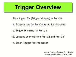
Trigger Overview. Planning for TN (Trigger Nirvana) in Run-04. Expectations for Run-04 Au-Au Luminosities Trigger Planning for Run-04 Lessons Learned from Run-02 and Run-03 Smart Trigger Pre-Processor. Jamie Nagle – Trigger Coordinator University of Colorado at Boulder.

E N D
Trigger Overview • Planning for TN (Trigger Nirvana) in Run-04. • Expectations for Run-04 Au-Au Luminosities • Trigger Planning for Run-04 • Lessons Learned from Run-02 and Run-03 • Smart Trigger Pre-Processor Jamie Nagle – Trigger Coordinator University of Colorado at Boulder
Run-4 Au-Au Projections Wide parameter space: L(peak) = 4 x 10^26 2500 Hz AuAu L(peak) = 8 x 10^26 5000 Hz AuAu L(peak) = 16 x 10^26 10000 Hz AuAu maximum from Roser Plan Z-Vertex Loss 30% (often seen in previous runs) 50% (sometimes seen in previous runs) 75% (high level expectation) Beam store fill for 5 hours, with 2 hour lifetime. Peak BBCLL1 rates within |zvtx| < 30 cm 1250 Hz (L=4x10^26) & (zeff=50%) 2500 Hz (L=8x10^26) & (zeff=50%) 3750 Hz (L=8x10^26) & (zeff=75%) 5000 Hz (L=16x10^26) & (zeff=50%) 7500 Hz (L=16x10^26) & (zeff=75%)
* 24% loss of integrated luminosity from 30 minute start up time of HV/DAQ/etc. If we achieve the middle luminosity scenario and can archive* (with compression) the equivalent of 500 MB/s, we can record all data with BBCLL1 “Minimum Bias” triggers. This assumes all bandwidth to Min.Bias and 0.25 MB/event size. In this case, Level-2 is important for monitoring and filtering, but not triggering. L=8x10^26 & zeff=75% L=8x10^26 & zeff=50% L=4x10^26 & zeff=50%
Run A Run B Run C Au-Au Challenge Ahead I believe the most challenging case scenario will be archiving 250 MB/s (known technology) and the highest luminosity = 3000 Hz. Of course it could be more challenging. Key Example Values: Assume Red Case MB Event Size = 0.25 MB LVL2 Event Size = 0.4 MB 70% BW for MB 700 Hz archv. 30% BW for LVL2 190 Hz archv. Implies LVL2 rejection factor = (3000-700)/190 = 12 L=8x10^26 & zeff=75% L=8x10^26 & zeff=50% L=4x10^26 & zeff=50%
Run A Run B Run C Run Totals Model of dividing each store into three runs. Run A – MB Forced Accept Value = 4 LVL2 Rejection = 12 Run B – MB Forced Accept Value = 2 LVL2 Rejection = 4 Run C – MB Forced Accept Value = 1 LVL2 Rejection = none In a 20 week run, with 15 weeks of Au-Au production Two 5-hour stores per day = 40% RHIC eff. Additional 50% PHENIX eff. RUN A – MB = 2.7E8 LVL2SAMP = 1.1E9 RUN B – MB = 3.0E8 LVL2SAMP = 6.0E8 RUN C – MB = 2.7E8 LVL2SAMP = 2.7E8 ----------------- --------------------------- Total MB = 0.8E9 LVL2SAMP = 2.0E9 = 116 mb-1 = 315 mb-1 L=8x10^26 & zeff=75% L=8x10^26 & zeff=50% L=4x10^26 & zeff=50% Only a factor of 3 difference !
A Simple Plan In Run-2 we used 20-30% of the bandwidth for Minimum Bias triggers, and had a wide array of Level-2 algorithms to enhance various physics topics. Lessons learned: Many of these algorithm results have not been used 1 ½ years later. Various efficiencies degrade these triggered events relative to minimum bias. We have a limited time budget and manpower effort for Level-2 triggers. Proposal (see emails from Tony and Akiba and others): For Run-4 Au-Au use 70% of the bandwidth for Minimum Bias triggers. Select a few key physics topics that meet the following criteria: 1. Physics significantly benefits from additional factor of 3 in statistics 2. High efficiency Level-2 trigger algorithm can be developed 3. People are interested and willing to put in the work up front Each Level-2 trigger would need to have > 50 rejection factor.
A Simple Plan goes bad….. Short List • J/y mmand higher mass muon pairs • J/y ee and higher mass electron pairs • High pT photons (for example > 3.5 GeV – see work by Justin Frantz) • muons at high pT Single • f mm (i.e. two short MUID roads) • Single electron at high pT • Electron-muon coincidence • Aerogel trigger for high pT protons/antiprotons • High pT hadrons for correlation analyses • You get the idea……
Run-2 Muon Experience Newby, Cianciolo led the Level-2 Effort L2MuDiMuonTrigger: required 2 deep roads (lose 25% for J/y) excluded upper panel not shielded (lose 30% for J/y) Expected rejection for AuAu minimum bias ~ 58 Low luminosity observation ~ 40 High MUID occupancy was associated with collisions. High luminosity this degraded, but also the MUID HV fell off the plateau. Shielding is critical CPU time limitations for algorithms Local Level-1 trigger helps Smart Trigger Pre-Processors
Run-2 Level-2 Trigger Mix L2MuDiMuonTrigger: required 2 deep roads (lose 25% for J/y) excluded one small panel not shielded (lose 30% for J/y) Expected rejection for AuAu minimum bias ~ 58 Low luminosity observation ~ 40 High luminosity this degraded, but also the MUID HV fell off the plateau
Level-2 Time Budget DAQ Report: Plan is for 128 node event builder in Run-4 with absolute minimum bandwidth of 3 kHz. This allows for ~ 90 Assembly and Trigger Processor nodes, each with dual-CPU. Thus, at 3 kHz, with 180 CPU, there is 60 milliseconds per event. If we really only run 3 algorithms, that allows for 20 milliseconds per event. This is probably optimistic since ATP’s have other calls on their CPU, in particular if we employ compression.
L2 Muon Plots Effort led by Silvermyr, Nagle, Kelly and others. With simple parameterization from gap coordinate in station 2 and 3, one can reconstruct the invariant mass. This gave sufficient projected rejection for d-A. Resolution is dominated by method, and thus one can just use the middle of the peak strip rather than determining the true hit position. This method yields ~ 20-25% momentum resolution. Must use local tangent vectors in order to improve to the 5% level.
MUID Local Level-1 and BLT North arm MUIDLL1 funding is approved. Funding for extension of algorithm to include “short” roads is approved. John will give the status of performance this run and plans for next run. Blue Logic MUID Trigger has played a crucial role. Issues of timing, stability, and monitoring make this a less than ideal replacement for LL1. Blue Logic granularity is useful in proton-proton and deuteron-gold, but not very useful in Au-Au reactions.
Smart Trigger Pre-Processor People: Cheng-Yi Chi, JN, Bill Sippach (engineering) Purpose: (1) Calculate trigger primitives for Level-2 algorithms - sort data that spans individual DCM DSP’s - apply first calibrations and reduce data to x, E, t, … (2) Significant additional data buffering (3) Merge frames between DCM’s for SEB input Modification to data output stream P P C D C M D C M D C M D C M D C M D C M D C M P A R 2 Frame I: Raw data from all DCM Frame II: Calibrated data (Q values) Frame III: Clustered data (x offsets)
Prototype Board in Boulder Ability to run in identical mode to current Partitioner Module Additional output via channel link Channel link for future use LVDS output to jSEB Busy cable output Level-1 data input
MUTR Sorting and Calibrating • DCM DSP needs to calculate quick calibrated values. • e.g. MUTR – input 4 ADC values for each hit strip • output single Q value for each hit strip • Q = gain x (ADC sample 2) • additional DSP program speed constraint (first test looks okay) • PAR II is funded for Run-4 for the MUTR system only, but future includes processing for EMC, RICH, and possibly others. • PAR II for MUTR case: • Sorts strip data for each arm, station, • plane, gap, halfoctant • Finds clusters (2-3 contiguous hit strips • above zero suppression) • Fast x offset calculation using lookup table • based on Q(peak)/Q(total) • Output set of coordinate projections for • use in fast tracking algorithm
Schedule First prototype module has been tested at Nevis over the last month. Test setup at Boulder available and second prototype now in Boulder. Need 3.3 Volts for crates with MUTR in Run-4. Plan to have PAR II test in original PAR mode in July, including communication to jSEB, data pass through, busy, level-1 input. Test suite of software to check trigger primitive calculations in the next two months. Full integration into Run Control software in August/September. - gain filenames available in current pcf files - need other downloadable tables for PAR II (offset lookup) - extra setting option (-D) from run control to turn things on
My office Sean’s office Come visit us in Boulder !