Evolutionary Computing

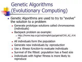
1. Evolutionary Computing • Consider the spectacular results of biological evolution • Designs better than any other known • Adaptive to changing requirements • Natural Selection works the same way regardless of the application • Algorithm is relatively unaware of application • Making it “more” aware may improve performance

2. Evolutionary Computing (Limitations) • Simulation of Natural Selection On a Smaller Scale • Can’t wait millions of years for evolution • Computer are fast and getting faster • EC works well on distributed computer architectures • Population sizes are much more limited • Actual evolutionary process is very complex – we can only approximate the process • Process is not fully understood • More accurate approximation requires additional computation resources

3. Simple Genetic Algorithms General Technique for multi-variable function optimization and machine learning Example: Design an airplane wing Variables: length, width, rotation in x-axis, rotation in y-axis

4. Example – Design an airplane wing Variables • Wing length (l) • Wing Width (w) • Sweep Angle (s) • Pitch Angle (p)

5. Fitness Function for Airplane Wing • Fitness(l,w,s,p) = Efficiency(l,w,s,p) = lift(l,w,s,p) / drag(l,w,s,p) • This is an extreme simplification, and I don’t know anything about designing airplane wings, but an aerospace engineer can give us the proper input variables and efficiency functions and that is what we would use. • Real case would have many more variables and a complex fitness function – perhaps a wind tunnel simulation.

6. What is the Range of Each Variable? • Length • Range 0 to 16 meters • 4-bits provides a 1 meter resolution • 5-bits would provides a .5 meter resolution • Width • Range 0 to 8 feet • 3-bits provides a 1 foot resolution • Sweep angle • Range 0 to 180 Degrees • 4-bits provides a 180/16 degree resolution • Pitch angle • Range -90 to 90 degrees • 5-bits provides a 180/32 degree resolution

7. Genetic Representation of Airplane Wing • 4 bits for length • 3 bits for width • 4 bits for sweep angle • 5 bits for pitch angle • Total of 16 bits to describe all 4 variables • Any random 16 bit value completely describes particular values for an airplane wing.

8. Create a population of random airplane wing strings • Select a population size. • Let’s use 500 for our airplane wing. • Create 500 random 16-bit values. • Each 16-bit value represents the string for an experimental aircraft wing • The fitness function can provide a measure of the quality of each of or 500 experimental wings • Because the values were generated randomly, most wings will be pretty bad and have low fitness values, but some will be better than others

9. Terminology • String - Sequence of genetic information fully describing an individual in the population. • Gene – location of a bit on a string • Allele – value of a gene

10. Natural Selection • As in the natural world • The more fit members of the population have a greater probability of propagating their genes into the next generation

11. Creating the Gene Pool for the Next Generation • More fit members should be more prominent in the gene pool • Less fit members should not be completely excluded • Excluding the less fit might remove important gene subsequences from the gene pool • Converging too quickly to a solution can provide suboptimal results

12. Reproduction • Select 500 members of the gene pool where the probability of the ith member of the population being selected is:

13. Reproduction (continued) • Once the 500 members of the gene pool for the next generation is established, pairs of parents are selected randomly. To distinguish between the two parents we will designate one as the father and the other as the mother, although their functions are identical.

14. Reproduction (continued) • Each pair of parents creates two children using one of two methods • Cloning • One child is an exact copy of the father • One child is an exact copy of the mother • Crossover • Some bits are copied from the mother, some from the father • Copy from one parent until you reach a crossover point, then copy from the other parent.

15. Crossover with Single Crossover Point ↓ • Father • Mother • Child 1 • Child 2

16. Crossover with Three Crossover Points ↓ ↓ ↓ • Father • Mother • Child 1 • Child 2

17. Mutation • Each bit copied to a child has a probability of being changed (from 1 to 0, or 0 to 1). • Usually the probability of mutation is relatively low, but enough to encourage diversity. • In other models, mutation is the principal method of genetic change.

18. Summary of Simple Genetic Algorithm • Create a population of random genes • For a specified number of generations • Apply the fitness function to each member of the population • Biasing toward the more fit individuals, create a pool of parents • While there are not a number of children equal to the original population size • Randomly select two parents and create two children either using cloning or crossover • Apply mutation • Completely replace the current generation with the children

19. Basic Parameters for a Genetic Algorithm • Population size • Gene Length • Number of crossover points • Probability of using crossover vs. cloning • Number of generations • Scaling Factors • More Complex/ Powerful applicatoin specific modifications

20. Schema • A Schema is a similarity template describing a subset of strings with similarities at certain string positions • Consists of series of 1’s, 0’s, and *’s (for don’t care) • Examples: • 1** • Matches (100, 101, 110, 111) • *10** • Matches (01000, 01001, 01010, 01011, 11000, 11001, 11011, 11011) The plural of the word schema is schemata.

21. Counting Schemata • For a binary schema of length k, there are 3k possible schemata • Each position may contain 0, 1, or * • A binary string of length k can have membership in 2k different schemata • Each position can contain the actual string digit, or * • Example • 101 has membership in schemata (101, 10*, 1*1, 1**, *01, *0*, **1, ***) • Schemata per populations • Range from 2k (all strings are the same) to n*2k (all strings have different schemata)

22. Schema Terms • Schema order o(H) is the number of fixed values • Number of 1’s and 0’s • 0**10 has an order of 3 • 0*1*11* has an order of 4 • Schema defining lengthδ(H) is the distance between first and last fixed value • Number of positions where crossover can disrupt the schema • 0**10 has a defining length of 4 • 0*1*11* has defining length of 5 • **1*1*1 has a defining length of 4 • 00**01*0 has a defining length of 7

23. f ( H ) + = m ( H , t 1 ) m ( H , t ) f Effect of Reproduction on Expected Number of Schemata in Population • A particular schema grows as the ratio of average fitness of the schema to average fitness of the population • m examples of a particular schema H at time t is m(H, t)

24. + ( f c f ) + = = + m ( H , t 1 ) m ( H , t ) ( 1 c ) * m ( H , t ) f Reproduction of Fit Schemata Suppose a particular schema H remains above average an amount c. Starting at t=0 and assuming a stationary value of c, we obtain Reproduction allocates exponentially increasing and decreasing numbers of schemata to future generations!

25. d ( H ) ³ - P 1 P * s c - l 1 Schema Disruption Due to Crossover • Ps = Probability of surviving crossover • Pd = Probability of being destroyed by crossover • Pc = Probability of crossover versus cloning • l is the length of the string • δ(H) is the defining length of the schema

26. Schema Disruption Due to Mutation • Pm = Probability of mutating each bit • o(H) is the schema order (number of fixed values) Probability a particular schema is disrupted by mutation is (1-pm)o(H) For very small values of pm, we can approximate this to 1 – o(H)pm

27. Fundamental Theorem of Genetic Algorithms Short, low-order, above-average schemata receive exponentially increasing trials in subsequent generations.

28. Position of Bits on the Gene is Important • Allow this to evolve as well • Dynamically change the location of each bit of the gene • Inversion • Select subsequences of the gene and invert the data and the interpretation • Has no effect on the genetic content, just the way the information is stored. • Requires additional meta-information to be stored that describes the location of each bit.

29. Inversion Example Randomly select two points in the sequence for inversion. This example, uses 5 and 9. The bit numbers and the data are inverted. Now bits 4 and 9 are adjacent and less likely to be disrupted with crossover.

30. Inversion Complicates Crossover • How do we combine these two genes with different bit orders? • Insist that parents have same organization (not very good) • Discard if crossover yields duplicate bit numbers • Reorder one parent, chosen at random, to match the other • Reorder the less fit of the two parents to match the other

31. When Might GA provide a Good Solution? • Highly multimodal functions • Discrete or discontinuous functions • High-dimensional functions, including many combinatorial ones • Nonlinear dependence on parameters (interactions among parameters) – epistasis makes it hard for others • Often used for approximate solutions to NP-complete combinatorial problems From Introduction to Genetic Algorithms Tutorial, Erik D. Goodman, Gecco 2005

32. Flavors of Evolutionary Computing • Genetic Algorithms (GA) • Evolutionary Programming (EP) • Classifier Systems • Evolving Neural Networks • Genetic Programming (GP) • Artificial Life (AL)

33. Acknowledgement Schema theory equations from David E. Goldberg’s, Genetic Algorithms in Search, Optimization and Machine Learning.