Download
1 / 38
380 likes | 404 Views
Explore the fundamentals, development, and practical applications of Genetic Algorithms (GAs) in optimization problems, understanding fitness functions, selection processes, crossover, and mutation. Witness GA demonstrations and learn about their efficacy through case studies, such as UCLA's Morphology Project.

E N D
Genetic Algorithms • Developed by John Holland in ‘60s • Did not become popular until late ‘80s • A simplified model of genetics and evolution by natural selection • Most widely applied to optimization problems (maximize “fitness”)
Assumptions • Existence of fitness function to quantify merit of potential solutions • this “fitness” is what the GA will maximize • A mapping from bit-strings to potential solutions • best if each possible string generates a legal potential solution • choice of mapping is important • can use strings over other finite alphabets
Outline of Simplified GA • Random initial population P(0) • Repeat for t = 0, …, tmax or until converges: • create empty population P(t + 1) • repeat until P(t + 1) is full: • select two individuals from P(t) based on fitness • optionally mate & replace with offspring • optionally mutate offspring • add two individuals to P(t + 1)
Fitness-Biased Selection • Want the more “fit” to be more likely to reproduce • always selecting the best premature convergence • probabilistic selection better exploration • Roulette-wheel selection: probability relative fitness:
Crossover: Biological Inspiration • Occurs during meiosis, when haploid gametes are formed • Randomly mixes genes from two parents • Creates genetic variation in gametes (fig. from B&N Thes. Biol.)
offspring GAs: One-point Crossover parents
offspring GAs: Two-point Crossover parents
offspring GAs: N-point Crossover parents
Mutation: Biological Inspiration • Chromosome mutation • Gene mutation: alteration of the DNA in a gene • inspiration for mutation in GAs • In typical GA each bit has a low probability of changing • Some GAs models rearrange bits (fig. from B&N Thes. Biol.)
The Red Queen Hypothesis • Observation: a species probability of extinc-tion is independent of time it has existed • Hypothesis: species continually adapt to each other • Extinction occurs with insufficient variability for further adaptation “Now, here, you see, it takes all the running you can do, to keep in the same place.”— Through the Looking-Glassand What Alice Found There
Demonstration of GA:Finding Maximum ofFitness Landscape Run Genetic Algorithms — An Intuitive Introductionby Pascal Glauser<www.glauserweb.ch/gentore.htm>
Demonstration of GA:Evolving to Generatea Pre-specified Shape(Phenotype) Run Genetic Algorithm Viewer<www.rennard.org/alife/english/gavgb.html>
Demonstration of GA:Eaters Seeking Food http://math.hws.edu/xJava/GA/
Morphology Projectby Michael “Flux” Chang • Senior Independent Study project at UCLA • users.design.ucla.edu/~mflux/morphology • Researched and programmed in 10 weeks • Programmed in Processing language • www.processing.org
Genotype ⇒ Phenotype • Cells are “grown,” not specified individually • Each gene specifies information such as: • angle • distance • type of cell • how many times to replicate • following gene • Cells connected by “springs” • Run phenome: <users.design.ucla.edu/~mflux/morphology/gallery/sketches/phenome>
Complete Creature • Neural nets for control (blue) • integrate-and-fire neurons • Muscles (red) • decrease “spring length” when fire • Sensors (green) • fire when exposed to “light” • Structural elements (grey) • anchor other cells together • Creature embedded in a fluid • Run <users.design.ucla.edu/~mflux/morphology/gallery/sketches/creature>
Effects of Mutation • Neural nets for control (blue) • Muscles (red) • Sensors (green) • Structural elements (grey) • Creature embedded in a fluid • Run <users.design.ucla.edu/~mflux/morphology/gallery/sketches/creaturepack>
Evolution Population: 150–200 Nonviable & nonre-sponsive creatures eliminated Fitness based on speed or light-following 30% of new pop. are mutated copies of best 70% are random No crossover
Gallery of Evolved Creatures • Selected for speed of movement • Run<users.design.ucla.edu/~mflux/morphology/gallery/sketches/creaturegallery>
Why Does the GA Work? The Schema Theorem
* * * * * 0 1 1 0 0 0 0 . . . * * 0 * 1 * 1 1 1 0 1 0 1 1 0 0 1 0 . . . 1 1 0 * 1 0 a stringbelongs tomany schemata a schemadescribesmany strings 1 1 0 0 0 1 1 1 0 0 1 0 Schemata A schema is a description of certain patterns of bits in a genetic string 1 1 * 0 * *
The Fitness of Schemata • The schemata are the building blocks of solutions • We would like to know the average fitness of all possible strings belonging to a schema • We cannot, but the strings in a population that belong to a schema give an estimate of the fitness of that schema • Each string in a population is giving information about all the schemata to which it belongs (implicit parallelism)
Exponential Growth • We have discovered:m(S, t+1) = m(S, t) f(S) / fav • Suppose f(S) = fav (1 + c) • Then m(S, t) = m(S, 0) (1 + c)t • That is, exponential growth in above-average schemata
**1 … 0*** |d| Effect of Crossover • Let = length of genetic strings • Let d(S) = defining length of schema S • Probability {crossover destroys S}:pd d(S) / (l – 1) • Let pc = probability of crossover • Probability schema survives:
Effect of Mutation • Let pm = probability of mutation • So 1 – pm = probability an allele survives • Let o(S) = number of fixed positions in S • The probability they all survive is(1 – pm)o(S) • If pm << 1, (1 – pm)o(S) ≈ 1 – o(S) pm
The Bandit Problem • Two-armed bandit: • random payoffs with (unknown) means m1, m2 and variances s1, s2 • optimal strategy: allocate exponentially greater number of trials to apparently better lever • k-armed bandit: similar analysis applies • Analogous to allocation of population to schemata • Suggests GA may allocate trials optimally
Paradox of GAs • Individually uninteresting operators: • selection, recombination, mutation • Selection + mutation continual improvement • Selection + recombination innovation • fundamental to invention: generation vs. evaluation • Fundamental intuition of GAs: the three work well together
Race Between Selection & Innovation: Takeover Time • Takeover time t* = average time for most fit to take over population • Transaction selection: population replaced by s copies of top 1/s • s quantifies selective pressure • Estimate t* ≈ ln n / ln s
Innovation Time • Innovation time ti = average time to get a better individual through crossover & mutation • Let pi = probability a single crossover produces a better individual • Number of individuals undergoing crossover = pcn • Probability of improvement = pipcn • Estimate: ti ≈ 1 / (pcpin)
Steady State Innovation • Bad: t* < ti • because once you have takeover, crossover does no good • Good: ti < t* • because each time a better individual is produced, the t* clock resets • steady state innovation • Innovation number:
schema theorem boundary cross-competition boundary drift boundary mixing boundary Feasible Region pc successful genetic algorithm crossover probability ln s selection pressure
Other Algorithms Inspired by Genetics and Evolution • Evolutionary Programming • natural representation, no crossover, time-varying continuous mutation • Evolutionary Strategies • similar, but with a kind of recombination • Genetic Programming • like GA, but program trees instead of strings • Classifier Systems • GA + rules + bids/payments • and many variants & combinations…
Additional Bibliography • Goldberg, D.E. The Design of Innovation: Lessons from and for Competent Genetic Algorithms. Kluwer, 2002. • Milner, R. The Encyclopedia of Evolution. Facts on File, 1990. VB