Evolutionary Computing. Genetic Algorithms
440 likes | 907 Views
Evolutionary Computing. Genetic Algorithms. Basic notions The general structure of an evolutionary algorithm Main directions in evolutionary computing Genetic algorithms: Encoding Selection Reproduction: crossover and mutation. Evolutionary computing.

Evolutionary Computing. Genetic Algorithms
E N D
Presentation Transcript
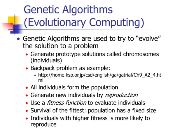
Evolutionary Computing. Genetic Algorithms • Basic notions • The general structure of an evolutionary algorithm • Main directions in evolutionary computing • Genetic algorithms: • Encoding • Selection • Reproduction: crossover and mutation Neural and Evolutionary Computing - Lecture 5
Evolutionary computing Evolutionary computing = design and application of techniques inspired by natural evolution Inspiration: evolution of species = • The species evolves by the development of new characteristics during reproduction caused by crossover and random mutations • In the evolutionary process the fittest individuals survive (those which are adapted to the environment) Problem solving = • Find a solution by searching the solution space using a population of potential candidates • The search is guided by a function which measures the degree of closeness to the solution Neural and Evolutionary Computing - Lecture 5
Evolutionary computing There are two main search mechanisms: • exploration = the search space is explored by the population elements which collect information about the problem • exploitation = the information collected during exploration are exploited and the potential solution(s) is refined Neural and Evolutionary Computing - Lecture 5
Evolutionary computing Search methods Neural and Evolutionary Computing - Lecture 5
Evolutionary computing Problem solving Information about the problem Configuration (candidate solution) Population of candidates Measure of the solution quality Exploitation mechanism Exploration mechanism Evolutionary process Natural environment Individual (chromosome) Population of individuals Fitness (degree of adaptation to the environment) Selection Reproduction (crossover and mutation) Neural and Evolutionary Computing - Lecture 5
Basic notions (1,0,0,1) {(0,0,0,0), (0,0,1,1), (1,0,0,1),(1,0,1,0)} {0,3,9,10} Chromosome = set of genes corresponding to an individual (potential solution for the problem) Population = finite set of individuals (chromosomes, candidate solutions) Genotype = the pool of all genes of an individual or population Phenotype = the set of all features represented by a genotype Neural and Evolutionary Computing - Lecture 5
Basic notions Ex: ONEMAX problem (1,0,0,1) 2 Crossover: (1,0,0,1) (1,0,1,1) (0,0,1,1) (0,0,0,1) Mutation: (1,0,1,1) (1,1,1,1) Fitness = measure of the quality of an individual (with respect to the problem to be solved) Generation = stage in the evolutionary process of a population (iteration in the search process) Reproduction = generation of offspring starting from the current population ( parents) by - crossover - mutation Neural and Evolutionary Computing - Lecture 5
Designing an Evolutionary Algorithm Components: Crossover Encoding Mutation Problem Evaluation Selection Neural and Evolutionary Computing - Lecture 5
Designing an Evolutionary Algorithm Population initialization Population evaluation REPEAT Parents selection Crossover Mutation Offspring evaluation Survivors selection UNTIL <stopping condition> Neural and Evolutionary Computing - Lecture 5
Directions in Evolutionary Computing Genetic Programming (Koza, 1990): Encoding: tree-like structures Crossover: main operator Mutation: secondary operator Applications: programs evolution Genetic Algorithms (Holland, 1962-1967): Encoding: binary Crossover: main operator Mutation: secondary operator Applications: combinatorial optimization Evolution Strategies (Rechenberg,Schwefel 1965): Encoding: real Mutation: main operator Recombination: secondary operator Applications: continuous optimization Evolutionary Programming (L. Fogel, D. Fogel, 1960-1970): Encoding: real / state digrams Mutation: the only operator Applications: continuous optimization Neural and Evolutionary Computing - Lecture 5
Applications Scheduling: vehicle routing problems, timetabling, routing in telecommunication networks Design: digital circuits, filters, neural networks Modelling: predictive models in economy, finances, medicine etc. Data mining: design of classification systems in engineering, biology, medicine etc. Neural and Evolutionary Computing - Lecture 5
Genetic algorithms • Encoding • Fitness function • Selection • Crossover • Mutation Neural and Evolutionary Computing - Lecture 5
Encoding Is a key element when a genetic algorithm is designed When an encoding method is used one have to take into account the problem to be solved Variants: • Binary encoding (the classical variant for GA) • Real encoding (appropriate for continuous optimization) • Specific encoding Neural and Evolutionary Computing - Lecture 5
Binary encoding Chromosome = binary sequence Search space: {0,1}n, n is given by the problem size Examples: • ONEMAX: find the binary sequence (x1,…,xn) which maximizes the function f(x1,…,xn)=x1+…+xn • Knapsack: there is a set of n objects of weights (w1,…,wn) and values (v1,…,vn) and a knapsack of capacity C; find a subset of objects which can be included in the knapsack without overpassing its capacity and such that the total value of selected objects is maximal Encoding: (s1,…,sn) si=0 object i is not selected si=1 object i is selected Neural and Evolutionary Computing - Lecture 5
Binary encoding • Optimization of a function defined on a continuous domain. f:[a1,b1]x...x[an,bn] R X=(x1,…,xn) V=(v1,…,vn) U=(u1,…un) Y=(y1,…,yn, yn+1,…ynr) vi=(xi-ai)/(bi-ai) (vi belongs to [0,1]) ui=[vi*(2r-1)] (ui is a natural number from {0,… 2r-1} => it can be represented in base 2 on r positions) (yn(i-1)+1,…yni) = binary representation of ui Neural and Evolutionary Computing - Lecture 5
Binary encoding Remark. The binary encoding has the disadvantage that close values can correspons to binary sequences with a large Hamming distance (ex. 7=(0111)2, 8=(1000)2) Solution: use of the Gray code (successive values have binary sequences which are different in only one position) (b1,…,br) (g1,…,gr) g1=b1 gi=(bi-1 + bi ) mod 2 Neural and Evolutionary Computing - Lecture 5
Binary encoding Gray code: (b1,…,br) (g1,…,gr) g1=b1 gi=(bi-1 + bi )mod 2 Decoding: bj=(g1+…+gj ) mod 2 Neural and Evolutionary Computing - Lecture 5
Particular encoding It is specific to the problem to be solved Example: permutation-like encoding (s1,s2,…,sn), si in {1,…,n}, si<>sj for all i<>j Problem: TSP si = index of the town visited at step i Remarks. It ensures the fact that the constraints are satisfied. Neural and Evolutionary Computing - Lecture 5
Fitness function Fitness - measures the quality of an individual - as the value of the fitness is larger the probability of the element to survive is larger Problem: unconstrained optimization The fitness function is proportional with the objective function (for a maximization problem) and inverse proportional with the objective function (for a minimization problem) Problem: constrained optimization The fitness function depends both on the objective function and on the constraints Neural and Evolutionary Computing - Lecture 5
Fitness function Constraints: included in the objective function by using the penalty method (no penalty if the constraint is satisfied) (the penalty is larger if the constraint is not satisfied ) Neural and Evolutionary Computing - Lecture 5
Fitness function Example: knapsack problem Fitness function Neural and Evolutionary Computing - Lecture 5
Selection Aim: - decide which of the elements from the current populations will be used to construct offspring (parents selection) - decide which of the elements from the offspring population will belong to the next generation (survivors selection) Basic idea: - the elements with a high fitness have a higher chance to be selected Selection mechanisms: - proportional selection - rank based selection - tournament selection - truncation selection Neural and Evolutionary Computing - Lecture 5
Proportional selection • Steps: • Compute the selection probabilities • Generate random values according to the distribution • 1 2 … m • p1 p2 … pm • Implementation: • (i) “Roulette Wheel” • (ii) “Stochastic Universal Sampling” (SUS) Current population: P=(x1,…,xm) Fitness values: (F1,…,Fm) Selection probabilities: pi=Fi/(F1+…+Fm) Rmk. If Fi are not strictly larger than 0 than they can be changed as follows: F’i=Fi-min(Fi)+eps Neural and Evolutionary Computing - Lecture 5
Proportional Selection Example: 1 2 3 4 0.2 0.4 0.3 0.1 Roulette Wheel (metoda ruletei) • Let us consider a roullete divided in m sectors having areas proportional to the selection probabilities. • Spin off the roulette and the index of the sector in front of the indicator gives the element to be selected from the population Neural and Evolutionary Computing - Lecture 5
Proportional selection • Rmk. • This algorithm corresponds to the simulation of a random variable starting from its distribution • One run gives the index of one element • To simultaneously generate the indices of several element the SUS (Stochastic Universal Sampling) variant can be used Implementation: Ruleta (p[1..m]) i:=1 s:=p[1] u:=random(0,1) while s<u do i:=i+1 s:=s+p[i] endwhile Return i Neural and Evolutionary Computing - Lecture 5
Proportional selection Algorithm: SUS(p[1..m],k) u:=random(0,1/k) s:=0 for i:=1,m do c[i]:=0 s:=s+p[i] while u<s do c[i]:=c[i]+1 u:=u+1/k endwhile endfor Return c[1..m] Stochastic Universal Sampling Idea: Rmk: k represents the number of elements which should be selected c[1..m] will contain the number of copies of each element Neural and Evolutionary Computing - Lecture 5
Proportional selection Disadvantages: • If the objective function does not have positive values the fitness values should be transformed • If the difference between the fitness value of the best element and that of other elements is large then it is possible to fill the populations with copies of the best element (this would stop the evolutionary process) Neural and Evolutionary Computing - Lecture 5
Rank based selection Particularities: the selection probabilities are computed based on the rank of elements in an increasingly sorted list by fitness Steps: 1.increasingly sort the fitness values 2. each distinct value in the list will have a rank (the smallest fitness value corresponds to rank 1) 3. divide the population in classes of elements having the same rank (e.g. k classes) 4. compute the selection probabilities: Pi= i/(1+2+…+k) 5. select classes using the roulette wheel or SUS methods; randomly select an element from each class. Neural and Evolutionary Computing - Lecture 5
Tournament selection Idea: an element is selected based on the result of a comparison with other elements in the population The following steps should be followed to select an element: • Randomly select k elements from the population • From the k selected elements choose the best one Remark. • Typical case: k=2 Neural and Evolutionary Computing - Lecture 5
Truncated selection Idea: from the joined population of parents and offspring the k best elements are selected Remark. • This is the only completely deterministic selection • It is mainly used for evolution strategies Neural and Evolutionary Computing - Lecture 5
Crossover Aim: combine two or several elements in the population in order to obtain one or several offspring Remark: in genetic algorithms there are usually two parents generating two children Variants: -one cut-point - uniform - convex - tailored for a given problem Neural and Evolutionary Computing - Lecture 5
Cut-points crossover Two cut points Parents Parents One cut point Children Children Neural and Evolutionary Computing - Lecture 5
Cut-points crossover Remarks: • For each pair of selected parents the crossover is applied with a given probability (0.2<=Pc<=0.9) • The cut points are randomly selected • Numerical experiments suggest that two cut-points crossover leads to better results than one cut-point crossover Neural and Evolutionary Computing - Lecture 5
Uniform crossover Particularity : the genes of offspring are randomly selected from the genes of parents Notations: x =(x1,…xn), y =(y1,…,yn) – parents x’=(x’1,…x’n), y’=(y’1,…,y’n) – offspring Neural and Evolutionary Computing - Lecture 5
Crossover for permutation – like elements Aim: include heuristic schemes which are particular Example: TSP (a tour is given by the order of visiting the towns) Parents: A B C D E F G Cutpoint: 3 A B E G D C F Offspring: A B C E G D F A B E C D F G Neural and Evolutionary Computing - Lecture 5
Mutation Aim: it allows to introduce new genes in the gene pool (which are not in the current genotype) Remark: the mutation depends on the encoding variant Binary encoding: the mutation consists of complementing some randomly selected genes Variants: • Local (at chromosome level) • Global (at gene pool level) Neural and Evolutionary Computing - Lecture 5
Mutation Chromosome level Steps: • Select chromosomes to be mutated (using a small mutation probability) • For each selected chromosome select a random gene which is mutated Remark: The mutation probability is correlated with the population size (e.g. Pm=1/m) Neural and Evolutionary Computing - Lecture 5
Mutation Pool gene level Assumptions: all chromosomes are concatenated, thus the form a long binary sequence Mutation: All genes are visited and for each one is decided (based on a mutation probability) if it is mutated or not Remark: • This variant allows to change several genes of the same chromosome Neural and Evolutionary Computing - Lecture 5
Mutation Permutation encoding: TSP Example: 2-opt transformation C C D D B B E E A A F F G G ABCDEFG ABCFEDG ABCFEDG Neural and Evolutionary Computing - Lecture 5