Download

1 / 68
790 likes | 1.04k Views
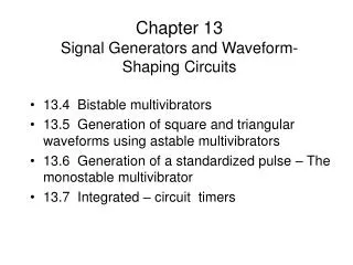
Signal Generators and Waveform-Shaping Circuits. 1.

E N D
Signal Generators and Waveform-Shaping Circuits 1
Figure 13.1 The basic structure of a sinusoidal oscillator. A positive-feedback loop is formed by an amplifier and a frequency-selective network. In an actual oscillator circuit, no input signal will be present; here an input signal xs is employed to help explain the principle of operation.
Figure 13.2 Dependence of the oscillator-frequency stability on the slope of the phase response. A steep phase response (i.e., large df/dw) results in a samll Dw0 for a given change in phase Df (resulting from a change (due, for example, to temperature) in a circuit component).
Figure 13.3 (a) A popular limiter circuit. (b) Transfer characteristic of the limiter circuit; L- and L+ are given by Eqs. (13.8) and (13.9), respectively. (c) When Rf is removed, the limiter turns into a comparator with the characteristic shown.
Figure 13.4 A Wien-bridge oscillator without amplitude stabilization.
Figure 13.5 A Wien-bridge oscillator with a limiter used for amplitude control.
Figure 13.6 A Wien-bridge oscillator with an alternative method for amplitude stabilization.
Figure 13.8 A practical phase-shift oscillator with a limiter for amplitude stabilization.
Figure 13.9 (a) A quadrature-oscillator circuit. (b) Equivalent circuit at the input of op amp 2.
Figure 13.10 Block diagram of the active-filter-tuned oscillator.
Figure 13.11 A practical implementation of the active-filter-tuned oscillator.
Figure 13.12 Two commonly used configurations of LC-tuned oscillators: (a) Colpitts and (b) Hartley.
Figure 13.13 Equivalent circuit of the Colpitts oscillator of Fig. 13.12(a). To simplify the analysis, Cm and rp are neglected. We can consider Cp to be part of C2, and we can include ro in R.
Figure 13.15 A piezoelectric crystal. (a) Circuit symbol. (b) Equivalent circuit. (c) Crystal reactance versus frequency [note that, neglecting the small resistance r, Zcrystal = jX(w)].
Figure 13.16 A Pierce crystal oscillator utilizing a CMOS inverter as an amplifier.
Figure 13.17 A positive-feedback loop capable of bistable operation.
Figure 13.18 A physical analogy for the operation of the bistable circuit. The ball cannot remain at the top of the hill for any length of time (a state of unstable equilibrium or metastability); the inevitably present disturbance will cause the ball to fall to one side or the other, where it can remain indefinitely (the two stable states).
Figure 13.19 (a) The bistable circuit of Fig. 13.17 with the negative input terminal of the op amp disconnected from ground and connected to an input signal vI. (b) The transfer characteristic of the circuit in (a) for increasing vI. (c) The transfer characteristic for decreasing vI. (d) The complete transfer characteristics.
Figure 13.20 (a) A bistable circuit derived from the positive-feedback loop of Fig. 13.17 by applying vI through R1. (b) The transfer characteristic of the circuit in (a) is noninverting. (Compare it to the inverting characteristic in Fig. 13.19d.)
Figure 13.21 (a) Block diagram representation and transfer characteristic for a comparator having a reference, or threshold, voltage VR. (b) Comparator characteristic with hysteresis.
Figure 13.22 Illustrating the use of hysteresis in the comparator characteristics as a means of rejecting interference.
Figure 13.23 Limiter circuits are used to obtain more precise output levels for the bistable circuit. In both circuits the value of R should be chosen to yield the current required for the proper operation of the zener diodes. (a) For this circuit L+ = VZ1 + VD and L– = –(VZ2 + VD), where VD is the forward diode drop. (b) For this circuit L+ = VZ + VD1 + VD2 and L– = –(VZ + VD3 + VD4).
Figure 13.24 (a) Connecting a bistable multivibrator with inverting transfer characteristics in a feedback loop with an RC circuit results in a square-wave generator.
Figure 13.24 (Continued) (b) The circuit obtained when the bistable multivibrator is implemented with the circuit of Fig. 13.19(a). (c) Waveforms at various nodes of the circuit in (b). This circuit is called an astable multivibrator.
Figure 13.25 A general scheme for generating triangular and square waveforms.
Figure 13.26 (a) An op-amp monostable circuit. (b) Signal waveforms in the circuit of (a).
Figure 13.27 A block diagram representation of the internal circuit of the 555 integrated-circuit timer.
Figure 13.28 (a) The 555 timer connected to implement a monostable multivibrator. (b) Waveforms of the circuit in (a).
Figure 13.29 (a) The 555 timer connected to implement an astable multivibrator. (b) Waveforms of the circuit in (a).
Figure 13.30 Using a nonlinear (sinusoidal) transfer characteristic to shape a triangular waveform into a sinusoid.
Figure 13.31 (a) A three-segment sine-wave shaper. (b) The input triangular waveform and the output approximately sinusoidal waveform.
Figure 13.32 A differential pair with an emitter degeneration resistance used to implement a triangular-wave to sine-wave converter. Operation of the circuit can be graphically described by Fig. 13.30.
Figure 13.33 (a) The “superdiode” precision half-wave rectifier and (b) its almost ideal transfer characteristic. Note that when vI> 0 and the diode conducts, the op amp supplies the load current, and the source is conveniently buffered, an added advantage.
Figure 13.34 (a) An improved version of the precision half-wave rectifier: Diode D2 is included to keep the feedback loop closed around the op amp during the off times of the rectifier diode D1, thus preventing the op amp from saturating. (b) The transfer characteristic for R2 = R1.
Figure 13.35 A simple ac voltmeter consisting of a precision half-wave rectifier followed by a first-order low-pass filter.
Figure 13.37 (a) Precision full-wave rectifier based on the conceptual circuit of Fig. 13.36. (b) Transfer characteristic of the circuit in (a).
Figure 13.38 Use of the diode bridge in the design of an ac voltmeter.
Figure 13.39 A precision peak rectifier obtained by placing the diode in the feedback loop of an op amp.
Figure 13.42 Example 13.1: Capture schematic of a Wien-bridge oscillator.
Figure 13.43 Start-up transient behavior of the Wien-bridge oscillator shown in Fig. 13.42 for various values of loop gain.
Figure 13.44 Example 13.2: Capture schematic of an active-filter-tuned oscillator for which the Q of the filter is adjustable by changing R1.
Figure 13.45 Output waveforms of the active-filter-tuned oscillator shown in Fig. 13.44 for Q = 5 (R1 = 50 kW).