Download
1 / 31
310 likes | 392 Views
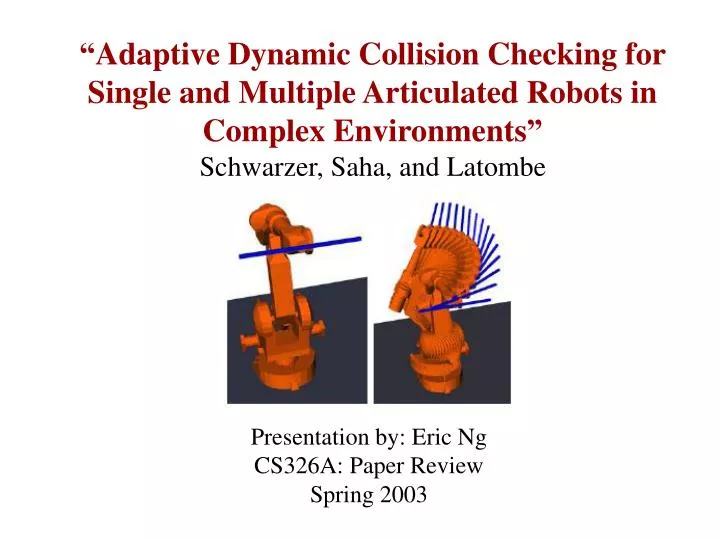
“Adaptive Dynamic Collision Checking for Single and Multiple Articulated Robots in Complex Environments” Schwarzer, Saha, and Latombe. Presentation by: Eric Ng CS326A: Paper Review Spring 2003. Static Collision Checking.

E N D
“Adaptive Dynamic Collision Checking for Single and Multiple Articulated Robots in Complex Environments” Schwarzer, Saha, and Latombe Presentation by: Eric Ng CS326A: Paper Review Spring 2003
Static Collision Checking • Static collision checking tests a single configuration of objects for overlaps. Aj Ai(q)
Dynamic Collision Checking • Dynamic collision checking ensures that all configurations between A and B are collision-free. • Fixed Resolution checking is a sequence of static BVH checks along path of motion, divided into length segments. • is user defined and is function of accuracy and calculation time.
Dynamic Collision Checking • Dynamic collision checking ensures that all configurations between A and B are collision-free. • Fixed Resolution checking is a sequence of static BVH checks along path of motion, divided into length segments. • is user defined and is function of accuracy and calculation time. B A
Fixed Resolution Collision Checker • Dynamic collision checking ensures that all configurations between A and B are collision-free. • Fixed Resolution checking is a sequence of static BVH checks along path of motion, divided into length segments. • is user defined and is function of accuracy and calculation time. B A
Fixed Resolution Collision Checker • Dynamic collision checking ensures that all configurations between A and B are collision-free. • Fixed Resolution checking is a sequence of static BVH checks along path of motion, divided into length segments. • is user defined and is function of accuracy and calculation time. B A
Fixed Resolution Collision Checker • Dynamic collision checking ensures that all configurations between A and B are collision-free. • Fixed Resolution checking is a sequence of static BVH checks along path of motion, divided into length segments. • is user defined and is function of accuracy and calculation time. B A e
q1 Undetected obstacle q2 q2 e q1 Drawbacks of Fixed Resolution Checking (1) determines accuracy. If isn’t fine enough, collision at a point between checks will not be detected. (2) Refining resolution improves accuracy, but calculation becomes more expensive.
Why Adaptive Dynamic Checking? Adaptive Dynamic Checking offers: (1) Ability to never miss collisions. (2) And not costing much more than classical collision checking. (3) Has one drawback: requires calculation of distances between objects, not just collision checking => can be computationally expensive. (Ameliorated with optimizations!)
Basis for Adaptive Dynamic Collision Checking • The robot and obstacles are defined by: A1,…,An, whose placement in workspace is q=(q1,…,qn) Aj Ai(q)
Basis for Adaptive Dynamic Collision Checking • nij(q) is lower bound distance between Ai and Aj h(q) Aj Ai(q)
i(q1,q2) Ai(q1) Aj(q2) Basis for Adaptive Dynamic Collision Checking • nij(q) is lower bound distance between Ai and Aj i(q1,q2) is upper bound path length of Ai from config 1 to 2. h(q) Aj Ai(q)
Basis for Adaptive Dynamic Collision Checking If i (qa,qb) + j (qa,qb) < nij (qa) + nij (qb), then there exists no collisions between qa and qb Lemma i (qa,qb) j (qa,qb) qa nij (qb) qb qa qb nij (qa) Ai Aj
What if Inequality Fails? • It does not mean there is a collision between “a” and “b”!! • Inequality only determines non-collisions. • Collision is defined by zero distance between Ai and Aj, ie: nij=0. nij(qb)=0 qa qa qb qb Aj Ai
Example of Adaptive Bisection of Paths • Run Inequality test on path segment. [PASS] = no collisions between qa and qb qa qb
Example of Adaptive Bisection of Paths • Run Inequality test on path segment. [PASS] = no collisions between qa and qb [FAIL] = check if robot makes collision at qmid If qmid doesn’t have a collision, recursively test both sub-segments until collision is found, or both sub-segments pass inequality test ==> never misses collision! Run Inequality Test qa qmid qb
Example of Adaptive Bisection of Paths • Run Inequality test on path segment. [PASS] = no collisions between qa and qb [FAIL] = check if robot makes collision at qmid If qmid doesn’t have a collision, recursively test both sub-segments until collision is found, or both sub-segments pass inequality test ==> never misses collision! Run Inequality Test qa qmid qb
i(q1,q2) Ai(q1) Aj(q2) Calculating the terms in the Inequality • i (qa,qb) + j (qa,qb) < nij (qa) + nij (qb) • But how do we get nij and i (qa,qb)? h(q) Aj Ai(q)
Object i Object j Half,i1 Half,j1 Half,i2 Half,j2 Leaf,i1 Leaf,i2 Leaf,j1 Leaf,j2 Computing Lower Bound Dist. Betw. Objects: nij • = distance(Object i,Object j) • If > 0, then return • Else, we need to investigate further Algorithm GREEDY-DIST(Bi, Bj)
Object i Object j Half,i1 Half,j1 Half,i2 Half,j2 Leaf,i1 Leaf,i2 Leaf,j1 Leaf,j2 Computing Lower Bound Dist. Betw. Objects: nij = 0 > 0 • Test both Half,j1 and Half,j2 against Object i • Dist1 = Greedy-Dist(Object I, Half,j1) • Dist2 = Greedy-Dist(Object I, Half,j2) • Dist2 > 0 (stop in that search path) • Dist1 !> 0 (need to continue further) = 0 Algorithm GREEDY-DIST(Bi, Bj)
Object i Object j Half,i1 Half,j1 Half,i2 Half,j2 Leaf,i1 Leaf,i2 Leaf,j1 Leaf,j2 Computing Lower Bound Dist. Betw. Objects: nij = 0 > 0 • Test Half,j1 against Half,i1 and Half,i2 • Dist1 = Greedy-Dist(Half,j1, Half,i1) • Dist2 = Greedy-Dist(Half,j1,Half,i2) • Both Dist1 and Dist 2 > 0 => DONE! • Return min(dist1, dist2) as nij = 0 Algorithm GREEDY-DIST(Bi, Bj)
A4 q4 A3 q3 q2 A2 A1 q1 Example of Bounding Motion Calculation: i D: dist by q3 • 4 d.o.f. robot • 3 rotational and 1 prismatic joint • D is the max distance travelled by • Q3 • L is the length of each rigid body L: length of each rigid body
Example of Bounding Motion Calculation: i Rigid Body Upper Bound Path Length A1 A1 q1
Example of Bounding Motion Calculation: i Rigid Body Upper Bound Path Length A1 A2 q2 A3 A2 A4 A1 q1
Example of Bounding Motion Calculation: i Rigid Body Upper Bound Path Length A1 A3 A2 q3 q2 A3 A2 A4 A1 q1
A4 q4 A3 q3 q2 A2 A1 q1 Example of Bounding Motion Calculation: i Rigid Body Upper Bound Path Length A1 A2 A3 A4
Conclusions • Adaptive Bisection Collision Checker is an efficient and robust way to determine if a proposed path is collision-free. • Even though it is efficient, there is room for improvement. For example, path lengths are overly conservatively computed. • Bisection method may not be most efficient solution when obstacle is always closeby the robot.
Optimizing the Process • Let Q be the priority queue containing elements objects being checked. • If the path segment is collision-free, then the ordering of Q has no impact on running time. But for a colliding path, the calculation can complete as soon as collision is found =>ordering matters. • Since longer path lengths have higher probability of collision, Q is presorted by decreasing path lengths to potentially find collisions earlier.
Comparative Experiment • SBL: PRM planner (single-query, bi-directional, lazy in cc) with fixed-discretization collision checker • A-SBL: Same planner, with new collision checkerExperiment: • Run SBL 10 times on same planning problem with some resolution e • If a collision has been missed, reduce e and repeat • If no collision has been missed, return average planning time • Run A-SBL 10 times and return average planning time Robot: 2,502 triangles Obstacles: 432 Triangles SBL 17 sec A-SBL 4.8 sec Slide courtesy Latombe,2003
More Results Robot: 2,502 triangles Obstacles: 432 Triangles SBL 17 sec A-SBL 4.8 sec Robot: 2,991 triangles Obstacles: 432 Triangles SBL 83 sec A-SBL 44 sec Robot: 2,991 trianglesObstacles: 74,681 triangles SBL 1.20 sec A-SBL 0.81 sec Robot: 2,502 trianglesObstacles: 34,171 triangles SBL 3.2 sec A-SBL 2.1 sec Robots: 6 x 2,991 trianglesObstacles: 19,668 triangles SBL 85 sec A-SBL 52 sec
Summary • Adaptive bisection collision checker is a reliable and effective way to test straight line segments. • Advantages over fixed resolution checker: • Never miss a collision • Eliminates need for determining resolution factor: • Determines whether subsections (“i” and “j”) of objects collide when moving from configuration “a” to “b” i (qa,qb) + j (qa,qb) < nij (qa) + nij (qb), does not collide • Requires lower bound distances between two bounding volumes (BVs) i & j at configs “a” & “b” • Requires upper bound distances in path lengths of objects i & j from config “a” to “b” • Inequality is performed on BVH binary tree until collision is found, or tree is fully traversed…leading to no collisions found