Download
1 / 91
910 likes | 920 Views
This article discusses the classical macro model of output determination, the role of the labour market, and the equilibrium in the labour market. It explores the demand and supply of labour, and the determinants of labour demand and supply. Economic intuition and mathematical derivations are used to explain the relationship between real wages and labour demand and supply.

E N D
The Classical Macro Model The Simple Classical Model
The Classical Assumptions • Classical economics stressed the role of real as opposed to nominal factors in determining real output. Money was only important as a medium of exchange. • Classical economics stressed the self-adjusting nature of the economy. Government policies to insure full employment were unnecessary and generally harmful. Classical economists assumed: • Perfectly flexible wages and prices. • Perfect information.
A Classical Model of Output Determination • The Starting point is the Production Function • Y = F(K, N) where • Y = National output • K = Capital • N = labour • And F is a functional notation • Assume K is constant in the short run so that Y varies directly with N. So to determine output, we need to know what determines employment, N. Employment is determined from the labour market. • In the labour market, we have the demand and the supply sides.
Properties of the Production Function With K given, output varies directly with the level of N From the production function, we can compute the following: Marginal product of labour can be derived from the production function using calculus. FN=MPN=dF/dN=dY/dN>0 FNN=d2F/dN2<0 i.e. the economy is subject to the law of diminishing returns. Does the following production function exhibit these properties? Y=K0.5N0.5, K=1
The Labour Market Note: Firms demand labour services and households supply labour services. The labour market comprises a) The Demand for labour side b) The Supply of Labour side : ASSUMPTIONS 1. Firms are profit maximizers 2. Households maximize their utility 3. Firms take the price level and money Wage as given; households take the money wage as constant 4. The labour market is ALWAYS in equilibrium.
Demand for Labour Firms employ labour to maximise profits and the condition that must be met is: P.MPN=W (1) where; P= the price level of output MPN=marginal product of labour W= money/nominal wage. (1) can be rewritten in a familiar form: MPN= W/P (2). So for the firm to maximize profit, equations (1) and (2) must hold. In fact, the two equations are the same but their use depends on the question under consideration.
Demand for Labour Cont’d From equation 2, MPN= W/P, for the firm to maximize profit in hiring labour, it must employ labour at the point where the marginal product of the last worker equals the fixed money wage. Because of diminishing returns, we consider the falling segment (the downward sloping portion) of the MPN curve. The profit maximising level of labour demand can be graphically determined using equations 1 or 2 as shown in diagrams below.
The Demand for labour Curve • Producers are willing to hire up to the point where the real wage (W/P) = MPN. • Notice that in the range of diminishing returns, the demand curve for labour is downward sloping. • The demand for labour can be expressed in both real and nominal terms. Figure1: Production Function and Marginal Product of labour Curve
Real vs. Nominal • The demand for labour can be expressed in real terms, i.e., Figure 2a (Top) • Firms maximize profits where W/P = MPN. • Or, alternatively, firms maximize profits where W = MPN x P. Labour demand can be expressed in nominal terms, as in Figure 2b (Bottom) • We will use both, depending on the situation. Figure 2a labour Demand for a Firm in real Terms Figure 2b The Demand for labour in Nominal Terms
Determinants of the Demand for labour by firms We conclude from the two diagrams that labour demand is a negative function of the real wage meaning as the real wage increases, labour demand decreases and vice versa: Nd = f (W/P) (-) That is, the demand for labour is a negative function of the real wage, i.e., the higher the real wage, the lower the demand for labour. Can you use economic intuition to explain this? or,
Labour Supply Classical economists assumed that individuals maximize their utility or satisfaction. Utility was generated by real income earned through the disutility of work that could then be used to purchase marketable goods and services as well as leisure. There is therefore a trade-off between real income resulting from working and the pleasures or utility of leisure, doing your own thing. U=f(Consumption, Leisure) with the following constraint: W+L=H, H=24 hours
Labour Supply Ns = g (W/P) (+) or, the supply of labour is a positive function of the real wage, i.e., the higher the real wage, the higher the supply of labour. Classicals believed that the substitution effect of a money wage change outweighed the income effect so labour supply increases when real wage increases. The opposite is also true : labour supply decreases when real wage decreases. So when plotted against the real wage, the labour supply curve is upward sloping.
Plotted against the real wage, an Individual Labour Supply Curve is upward sloping on
Equilibrium Output and Employment To determine what the equilibrium levels of employment and output will be in an economy, according to the classical model, we first of all get the employment level from the labour market (N*). With N determined, we put it into the production function and obtain equilibrium output (Y*). The following 4 equations are needed: 1. Nd= f (W/P) 2. Ns= g (W/P) 3. Ns = Nd 4. Y = F (K*, N)
Determinants of the Position of the Labour Supply Curve A change in population growth rate A change in preference for leisure as against working for more hours A change in the training content of institutions responsible for training potential labour supply.
Equilibrium in the labour Market • Equilibrium in the labour market yields the market real wage (W/P)0 and the level of employment (N0). • Given the (N0) level of employment, the level of income is determined at (Y0). • The economy automatically adjusts to full employment at (N0). Figure 3 Classical Output and Employment Theory
Numerical Illustration A classical economy is described by the following functions: Y=200KN-1/4N2 Ns=300+8W/P a) Derive the labour demand function and determine its slope. Assume K=1 b) Determine N*, (W/P)* and Y*. c) Provide a rough sketch of your answers.
Effect of a Change in Price • Price level change has no effect on real variables. • As P , W in the same proportion, so that (W/P) and N are unchanged. • Effect can be shown to be the same: no matter whether we use real wage (W/P) as in part a, or nominal wage (W) as in part b, price level changes have no real effect in the classical system. Figure 4 labour Market Equilibrium and the Money Wage
The Aggregate Supply Curve • If we plot various levels of prices (the absolute price level) and their respective level of Y, we plot out a vertical aggregate supply curve. • The level of real output is not affected by nominal variables. • Real output is affected only by real variables. Figure 5 Classical Determination of Aggregate Supply
Shifts in the Aggregate Supply Curve • A change in the level of capital stock is a change in a real factor. • As K, the production function shifts up, which shifts the labour demand curve, i.e., the MPN or Nd . • The real wage (W/P) and the real level of employment (N). • The level of real output is only affected by real variables. • Real output is not affected by nominal variables. Figure 6 The Effect on Output, the Real Wage, and Employment of an Increase in the Capital Stock in the Classical System
The Classical Macro Model Money in the Classical System
Classical Aggregate Demand • Classical economics is supply-side economics. • Real output on the supply side is determined by the real factors of production—land, labour, capital, and entrepreneurial ability. Y=F(K,N) is real! • All variables that are supply side determined are real variables—Y, N, MPN, W/P, S, I, C, r. • Autonomous variables, such as G and T are real. • The demand side is important only in determining the nominal variables—W, P, MPNxP. • The money supply, M, is a nominal variable. • The classical aggregate demand curve is an implicit aggregate demand. • What is the role of money in determining aggregate demand?
Determination of Price in the classical model To classical economists, the quantity of money determines the price level. That is, P=f(Ms). To determine the direction and the extent to which price depends on money supply, we need a theory: The Quantity Theory of Money of which two versions will be discussed – the Fisherien and; the Cambridge Versions. The building blocks for the 2 approaches is the equation of exchange: MV=PY
The Equation of Exchange MV=PY where; M= Quantity of money supply V= Velocity of money P= general or average price level Y= real output (quantity of goods & services an economy produces in a year) MV= Total value of money used to purchase goods in a year PY=total value of goods produced in a year MV=PY is a truism!
The Equation of Exchange & the Quantity Theory of Money To move from the EE to the QTM, we need to know how the variables in the EE are determined. ASSUMPTIONS M= money supply is exogenously determined by the central bank V= Velocity of money is fixed by institutional factors y= real output is determined by supply factors. To classical economists, y is fixed at the full employment level of output. With these assumptions, we can make P the subject of the expression: P=(MV)/Y
The Equation of Exchange & the Quantity Theory of Money • With V and Y fixed, their ratio is also fixed so P becomes a function of the quantity of money in a country. • INTERPRETATION: • P is directly proportional to M which means that: • 1. P increases whenever M increases and vice versa; • 2. P increases by the same proportion to M • If M increases by 10%, P increases by the same 10%, for example • If M increases by 40%, P increases by the same 40% In short, P is solely determined by money supply. This the quantity theory of money as expounded by Fisher. BUT HIS VERSION IS TOO MECHANICAL! WHAT IS THE ECONOMICS BEHIND IT?
The Cambridge Approach to the Quantity Theory In this version, we move away from the mechanical nature of the version of the QTM by Fisher. As championed by A. Marshall & A.C. Pigou , the QTM is put in the context of demand for money where the average money holdings is a constant fraction of nominal income: Md=k(Py), k>0 and 0<k<1
The Cambridge Approach to the Quantity Theory Cont’d We can move from the equation of exchange to money demand: k= 1/v From the money market equilibrium, an increase in Ms results in excess supply of money and excess spending and given the fixed output supply, prices will go up. This is the economics behind this version of this QTM: So the price level is determined by MS.
The Classical aggregate demand curve plots combinations of price level (P) and real output (Y) consistent with the equation of exchange, MV = PY, for a given money supply (M) and a fixed velocity (V). Assume M = 300 and V = 4. Points such as P = 12.0 and Y = 100 or P = 6.0 and Y = 200 (PY = 1200 = MV in each case) lie along the aggregate demand curve. An increase in the money supply to M = 400 shifts the aggregate demand curve to the right. Classical Aggregate Demand Figure 4-1 The Classical Aggregate Demand Curve
Deriving the AD Equation: We use the equation of exchange MV=PY to derive the classical AD equation. Since P and Y are variables and M and V are fixed constants, we can make P the subject of the equation above: Given M=300 and V=4, the ADC equation is : 300*4=PY 1200=PY (1) P=1200/Y (2) Thus, both (1) and (2) can be taken as ADC equation.
Successive increases in the money supply, from M1 to M2 and then to M3, shift the aggregate demand curve to the right, from Yd(M1) to Yd(M2) to Yd(M3). The price level rises from P1 to P2 to P3. Output, which is supply-determined, is unchanged (Y1 = Y2 = Y3). Effects of a Change in the Money Supply in the Classical System Figure 4.2 Aggregate Supply and Aggregate Demand in the Classical System
The Classical Theory of the Interest Rate • In the classical system, the equilibrium interest rate was the rate at which the amount of funds individuals & firms desired to lend was just equal to the amount of funds others desired to borrow. • The market in which the interest rate is determined is the Loanable Funds market or the Bonds market. • In this market, entities borrow by selling (issuing) bonds. By buying these bonds entities give out their savings or idle funds. • Like any market there ARE TWO SIDES: THE DEMAND & the SUPPLY SIDES • Household, firms and government constitute the demand side of the loanable funds market. • Household, firms and government also constitute the supply side of the loanable funds market.
The Classical Theory of the Interest Rate Cont’d • The SSLF may also be called the saving function or the demand for bonds • Similarly, the DDLF may also be called the Investment function or the supply of bonds • ASSUMPTIONS • 1. Classical economists assume that the LF market is always in equilibrium, i.e. SSLF=DDLF • 2. The interest rate is perfectly flexible. With excess demand for funds, the interest rate increases to clear the market and with excess supply the interest rate decreases. • This flexibility in the interest rate guarantees that exogenous changes in a particular component of AD do not affect the level of AD .
The SSLF and DDLF Schedules • At higher interest rate, people are enticed to save more so this gives an upward sloping SSLF schedule. • For the demand for Loanable funds curve, at higher interest rate, the cost of borrowing increases so demand for loanable funds will reduce so we postulate a downward sloping DDLF curve.
Demand and Supply of Loanable Funds Schedules • Putting the two together give the loanable funds market shown in Figure This market determines the amount borrowed and lent at the market equilibrium interest rate .
The Loanable Funds Theory of Interest Rates • The equilibrium interest rate (ro) is the rate that equates: • The supply of loanable funds consists of new saving (S), • The demand for loanable funds, which consists of investment (I) plus the bond-financed government deficit (G -T). Figure 4: Interest Rate Determination in the Classical System NOTE: The Loanable Funds Theory is a real theory of interest rates.
Changes in Autonomous Spending • An autonomous decline in investment shifts the investment schedule to the left from I0 to I1—the distance I. • The equilibrium interest rate declines from r0 to r1. • As the interest rate falls, there is an interest-rate-induced increase in investment—distance B. Figure 4.4 Autonomous Decline in Investment Demand
Changes in Autonomous Spending • There is also an interest-rated-induced decline in saving, which is an equal increase in consumption—distance A. • The interest-rate-induced increases in consumption and investment just balance the autonomous decline in investment. • There is no change in real output. Figure 4.4 Autonomous Decline in Investment Demand NOTE: A change in autonomous spending changes only the composition of output!
At point E, the equilibrium interest rate r0 equates the supply of loanable funds, S, with the demand for loanable funds, I. Adding government deficit spending, (G - T)1 shifts the demand for loanable funds to the right to point F. The interest rate rises from r0 to r1. Effect of Increase in Government Spending in the Classical Model Figure 4.5 Effect of Increase in Government Spending in Classical Model
The increase in the interest rate causes a decline in the quantity of investment from I0 to I1, a distance B, and an increase in saving, which is an equal decline in consumption, from S0 to Sl, a distance A. The decline in investment and consumption just balances the increase in government deficit spending, (G - T)1. Effect of Increase in Government Spending in the Classical Model Figure 4.5 Effect of Increase in Government Spending in Classical Model
Crowding Out • We have a name for what happens when the government increases its deficit. • It is called crowding out—100% crowding out or complete or total crowding out in the Classical case. • Govt spending crowds out private spending, partly from investors (less I) and partly from consumers (less C, that is to say, more S) • The level of output (Y) does not change. • The only change is in the composition of output. • Is that change real or nominal? • So we have seen that a bond-financed increase in G has no effect on output and employment!
Numerical Illustration You are given the following functions: (1) I = 58 - 7r (2) S = 8 + 3r (3) I = S a) Find r* and I* b) If the there is GHȼ30 million-bond financed increase in government expenditure, find: i) the new r* and I*. How will AD and Y be affected? Explain. ii) how much of investment is crowded out? How much of consumption is affected? Explain. iii) redo ii) using loanable funds diagrams.
Policy Implication of the classical Equilibrium Model Monetary policy Effects: Will monetary policy have real effects? That is, will it cause employment and output to change? The answer is no because the resultant change in price will not affect the real wage because the money wage will increase in proportion to the price level. So N, Y are not affected.
Increases in the money supply from M1 to M2 and then to M3, shift the aggregate demand curve to the right, from Yd(M1) to Yd(M2) to Yd(M3). The price level rises from P1 to P2 to P3. Output, which is supply-determined, is unchanged (Y1 = Y2 = Y3). Expansionary Monetary Policy Effects in the classical equilibrium model Figure 4.2 Aggregate Supply and Aggregate Demand in the Classical System
Fiscal Policy in the classical system Assume G goes up. We have to know how it is financed. There are 3 ways of raising the money: 1. Borrowing (increase in demand for loanable funds) – a bond-financed increase in G 2. Increase in Taxes (A Tax-financed increase in G) 3. Increase in money supply (Money-financed increase in G) For option 3, we already know the effect. Only prices will change but N, Y, Real wage, Interest rate will all not change. The AD curve will shift to the right on the vertical AS curve.
A bond-financed increase in G For a bond-financed increase in G, DDLF curve will shift to the right and at initial interest rate, there will be excess demand for funds so the interest rate increases. The increase in the interest rate has two effects on AD. 1. There is an interest rate induced fall in investment 2. With the interest rate increasing, saving will increase which is mirrored by an equal reduction in consumption (a component of AD)
A bond-financed increase in G Cont’d Because classical economists believed that the loanable funds market is always in equilibrium, the rise in the interest rate will cause reductions in consumption and investment whose magnitude will be equal to the initial increase in G. So on net there will be no change in AD; only that its components will change, consumption and Investment have reduced but G has increased. A bond-financed increase in G has no real effect!
The increase in the interest rate causes a decline in the quantity of investment from I0 to I1, a distance B, and an increase in saving, which is an equal decline in consumption, from S0 to Sl, a distance A. The decline in investment and consumption just balances the increase in government deficit spending, (G - T)1. A bond-financed Increase in Government Spending in the Classical Model Figure 4.5 Effect of Increase in Government Spending in Classical Model