Download
1 / 30
300 likes | 419 Views
The Basic Macro Model . The first examination of our primary theory and model to describe the economy and predict effects. The model itself is known as the Aggregate Demand- Aggregate Supply Model. Theories and Models.

E N D
The Basic Macro Model • The first examination of our primary theory and model to describe the economy and predict effects. • The model itself is known as the Aggregate Demand- Aggregate Supply Model.
Theories and Models • Theory -- An assertion about the major causes of observed behavior, done in order to predict outcomes. • Model -- A formalization of a theory, done to make concisepredictions.
The Aggregate Demand-Aggregate Supply Model • Purpose -- seeks to predict the behavior of real GDP (Y) and the price level (P) (and therefore inflation).
Aggregate Demand • Aggregate Demand (AD) -- the sum of all the newly produced US final goods and services that consumers, businesses, government, and foreigners intend to purchase (i.e. real GDP demanded).
Aggregate Demand: Causes • The Price Level (P) P (ceteris paribus) AD • Aggregate Expenditure (AE) -- desire to purchase quantities of newly produced final goods and services, apart from price considerations. AE (ceteris paribus) AD
Formalizing the Theory of Aggregate Demand • Graph AD versus one of its causes -- the price level (P). • Inverse relationship implies that the curve is downward sloping. • Changes in P are described as a movement along the curve. • Graph is drawn assuming that AE (and any other causes) are constant (ceteris paribus).
Describing Changes in One of the “Other Causes” • AE changes (or changes in any cause other than the price level) are described by a shift of the Aggregate Demand curve. • Contrast this with changes in P -- movement along the curve. • Different descriptions occur only because P is the cause that appears on the graph.
Shifting the AD Curve • Changes -- other than P -- that make AD increase are described as a rightward shift of the curve, or an increase in AD. • Changes -- other than P -- that make AD decrease are described as a leftward shift of the curve, or a decrease in AD.
A Brief Look at Aggregate Expenditure (AE) AE = C + I + (G - T) + (X - M) • AE: close to definition of real GDP. except that it subtracts out taxes. • Increases in C, I, G, or X increase AE (and therefore increase AD). • Increases in T or M decrease AE (and therefore decrease AD).
Aggregate Expenditure (AE) -- Continued AE = C + I + (G - T) + (X - M) • The causes of AE are the causes of C, I, (G - T), and (X - M) -- next chapter. • A change in any of them will shift the AD curve.
Short-Run Aggregate Supply (AS) • Short-Run Aggregate Supply (AS) -- the sum of all the newly produced US final goods and services that firms wish to produce (real GDP supplied), given inflexible input prices.
Short-Run Aggregate Supply -- Causes • Price Level (P) P AS • Price of Energy (PE) PE AS • The Nominal Wage Rate (W) W AS • Other Production Related Causes (e.g. labor productivity)
Short-Run Aggregate Supply: Formalizing • Graph AS versus one of its causes -- the price level (P). • Positive relationship implies that the curve is upward sloping. • Changes in P are described as a movement along the curve. • Graph is drawn assuming that PE, W, and any other causes are constant (ceteris paribus).
The Shape of the AS Curve • Describes different magnitudes ofresponse to increases in the price level (P). • k segment -- P increase generates large output response. • l segment -- P increase generates moderate output response. • m segment -- P increase generates small output response.
Describing Changes in One of the “Other Causes” • Changes in PE, W, or changes in any cause other than the price level are described by a shift of the AS curve. • Like Aggregate Demand, different descriptions occur only because P is the cause that appears on the graph.
Shifting the AS Curve • Changes -- other than P -- that make AS increase are described as a rightward shift of the curve, or an increase in AS. • Changes -- other than P -- that make AS decrease are described as a leftward shift of the curve, or a decrease in AS.
Equilibrium: The Market in Action • Equilibrium (Y* and P*) -- The values where real GDP and the price level will settle, given that the strategies of demands and suppliers play out.
Properties of Equilibrium • If the price level is anywhere else, natural market forces bring it to equilibrium. • P* and Y* represent the actual price level and real GDP predicted by the theory. • Shifts in either the AD or AS curves change the equilibrium.
Shifts and Changing the Equilibrium -- Applications • Example 1 -- The effect of a war on the economy. • War (G - T) • Increase in (G - T) increases AE, described by shifting the ADcurve rightward. • Draw the picture and evaluate the answer.
Another Application • Example 2 -- Firms become very pessimistic about the economy, decrease their purchases of new plants and equipment (1930s). • Decreased purchases of new plants and equipment I
Decrease in I also decreases AE, described by shifting the ADcurve leftward. • Draw the graphical situation and evaluate the answer.
Still Another Application • Example 3 -- The price of energy (PE) increases (energy crisis in US, 1970s). • PE hinders production, reduces Aggregate Supply. • Therefore the AS curve shifts leftward. • Draw the graphs and evaluate.
The “Nice Assumptions” -- Market Efficiency • No market power -- advantages in the market are transitory and can be eliminated by competition. -- equal access to information -- equal access to markets
No market failure -- markets function smoothly and quickly to coordinate choices. • Market failure in the economy -- nominal wage rates and energy prices do not adjust flexibly to macroeconomic conditions.
Market Failure in Macro • Market failure in Macro -- P changes, but W and PE stay constant. • Describes the upward sloping Aggregate Supply (AS) curve. • Main implication -- In the AD-AS model, Y* does not have to be equal to YF.
Characterizing the Economy (Short-Run) Y* < YF (sluggish economy, demand deficient unemployment) Y* > YF (accelerating inflation) Y* = YF (desired state of the economy)
Long-Run Aggregate Supply (LAS) • Long-Run Aggregate Supply (LAS) -- the sum of all the newly produced US final goods and services that firms wish to produce when all microeconomic adjustments have been completed under our nice assumptions(in particular, no market failure).
Characteristics of Long-Run Aggregate Supply (LAS) • Unaffected by the price level. • P W and PE as well no incentive for firms to change production plans. • Affected by production-oriented variables as well as peoples’ attitudes toward work (will study more later).
Formalizing Long-Run Aggregate Supply (LAS) • LAS curve is vertical when plotted against the price level (P). • Vertical at the full sustainable level of real GDP (YF), all adjustments completed under the “nice assumptions”. • Will consider shifts of the curve in a later chapter.
Putting The Model All Together -- Two “Teasers” • Teaser #1 -- The role of Economic Policy, getting Y* closer to YF. • Teaser #2 -- Spending gone too far, the wage-price spiral (nominal wage rates reacting to spending-induced inflation).