Download
1 / 16
160 likes | 168 Views
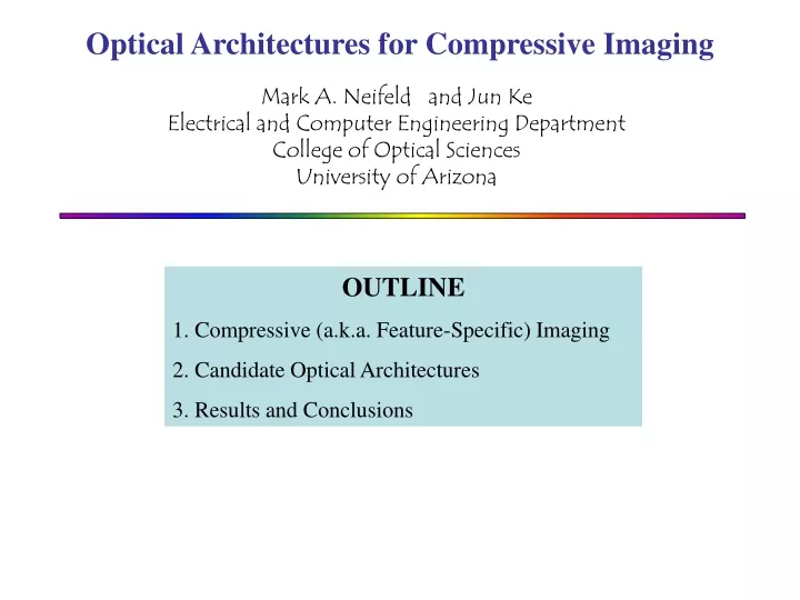
Optical Architectures for Compressive Imaging. Mark A. Neifeld and Jun Ke Electrical and Computer Engineering Department College of Optical Sciences University of Arizona. OUTLINE

E N D
Optical Architectures for Compressive Imaging Mark A. Neifeld and Jun Ke Electrical and Computer Engineering Department College of Optical Sciences University of Arizona OUTLINE 1. Compressive (a.k.a. Feature-Specific) Imaging 2. Candidate Optical Architectures 3. Results and Conclusions
Photons Object N - Detector Array Direct Image features M - Detector Array Object Compressive Imaging Conventional Feature-Specific • Conventional imagers measure a large number (N) of pixels • Compressive imagers measure a small number (M<<N) of features • Features are simply projections yi = (x∙ fi) for i = 1, …, M • Benefits of projective/compressive measurements include - increased measurement SNR improved image fidelity - more informative measurements reduced sensor power and bandwidth - enable task-specific imager deployment information optimal • Previous feature-specific imaging: Neifeld (2003), Brady (2005), Donoho (2004), Baraniuk (2005) random projections PCA, ICA, Wavelets, Fisher, … DCT, Hadamard, …
Feature-Specific Imaging for Reconstruction • PCA features provide optimal measurements in the absence of noise • Limit attention to linear reconstruction operators Noise-free reconstruction: PCA solution : General solution : photon count constraint depends on optics Result using PCA features:
FPCA RMSE = 12 RMSE = 11.8 FOPT RMSE = 12.9 RMSE = 124 What Happens in the Presence of Noise ? Problem statement with Noise: Stochastic tunneling to find optimal • PCA features are sub-optimal in the presence of noise. • PCA tradeoff between truncation error and measurement fidelity • Optimal features improve performance by - using optimal basis functions - using optimal energy allocation
Optimal Features in Noise • Optimal solution always improves with number of features • FSI results can be superior to conventional imaging • Optical implementation require non-negative projections
Feature-Specific Imaging Results Summary • Optimal FSI is always superior to conventional imaging • Non-negative solution is a good experimental system candidate • All these results rely on optimal photon utilization
N - Detector Array Noisy Measurements S y = x + n Object= x Imaging Optics Noise = n Candidate Architectures • Architecture Comparison Assumes • - Equal total photon number • - Equal total measurement time Architecture #1: Conventional Imaging Characteristics • All N measurements made in a single time step (noise BW ~ 1/T) • Photons divided among many detectors (measured signal ~ 1/N)
Noisy Measurement Single Photo-Detector Programmable Mask S n yi = fi x + n Object= x Light Collection Optics Imaging Optics Candidate Architectures Architecture #2: Sequential Compressive Imaging Characteristics • A single feature is measured in each time step (noise BW ~ M/T) • Photons collected on a single detector (measured signal ~ 1/M) • Unnecessary photons discarded in each time step (1/2) • Reconstruction computed via post-processing
Noisy Measurements Noise = n Fixed Mask S M – Detector Array Object= x {yi = fi x + n, i=1, …, M} Imaging m-Optics Candidate Architectures Architecture #3: Parallel Compressive Imaging Characteristics • All M features are measured in a single time step (noise BW ~ 1/T) • Photons collected on M << N detectors (measured signal ~ 1/M) • Unnecessary photons discarded in each channel (1/2) • Reconstruction computed via post-processing
y1 = f1 x + n y2 = f2 x + n Polarization Mask Re-Imaging Optics PBS PBS Imaging Optics Object= x n + n + Single Detector Candidate Architectures Architecture #4: Pipeline Compressive Imaging Characteristics • All M features are measured in a single time step (noise BW ~ 1/T) • Photons collected on M << N detectors (measured signal ~ 1/M) • No discarded photons most photon efficient • Most complex hardware • Reconstruction computed via post-processing
Architecture Comparison – Full Image FSI • All results use 80x80 pixel object. • All results use PCA features with optimal energy allocation among time/space channels. • All results use optimal linear post-processor (LMMSE) for reconstruction. • Measurement noise is assumed AWGN iid. Reconstruction RMSE versus SNR
Architecture Comparison – Full Image FSI • RMSE Trend 1: Pipeline < Parallel < Sequential • RMSE Trend 2: Compressive < Conventional for low SNR
Architecture Comparison – Blockwise FSI • Evaluate compressive imaging architectures for 16x16 block-wise feature extraction • All other conditions remain unchanged Reconstruction RMSE versus SNR • Block-wise operation shifts crossover to larger SNR • RMSE Trend 1: Pipeline < Parallel < Sequential • RMSE Trend 2: Compressive < Conventional for low SNR
Conclusions • Compressive imaging (FSI) exploits projective measurements. • There are many potentially useful measurement bases. • FSI can yield high-quality images with relatively few detectors. • FSI can provide performance superior to conventional imaging for low SNR. • Various optical architectures for FSI are possible. • FSI Reconstruction fidelity is ordered as Sequential, Parallel, Pipeline. • Pipeline offer best performance owing to optimal utilization of photons.