Optical Imaging (Some selected topics)

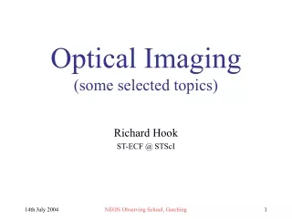
1. Optical Imaging(Some selected topics) http://www.stecf.org/~rhook/NEON/Arcetri_2007.ppt Richard Hook ST-ECF/ESO NEON Observing School, Arcetri

2. Some Caveats & Warnings! • I have selected a few topics, many things are omitted (eg, adaptive optics)! • I have tried to not mention material covered in other talks (detectors, photometry, spectroscopy…) • I am a bit biased by my own background, mostly Hubble imaging. • Mostly this talk refers to optical imaging, some things apply to near-IR imaging also and some things are more general. • I have avoided getting deep into technicalities so apologise if some material seems rather trivial. NEON Observing School, Arcetri

3. Topics of Talk • The imaging process • The optical system and its effects • The point-spread function • The pixel response function • Detectors: Artifacts, defects and noise characteristics • Basic image reduction • Image combination, dithering and drizzling • FITS format and metadata • Colour • Software - the Scisoft collection NEON Observing School, Arcetri

4. Two Examples:The power of imaging A supernova at z>1 detected in the Great Observatories Origins Deep Survey (GOODS). z-band imaging with Hubble ACS/WFC at multiple epochs. Public data: www.stsci.edu/science/udf A small section of the Hubble Ultra Deep Field (HUDF). The deepest optical image of the sky ever taken (i=31). 800 orbits with HST/ACS/WFC in BViz filters. Final scale 30mas/pix, format of entire image 10500x10500 pixels, FWHM of stars in combined image 80mas. Public data: www.stecf.org/UDF NEON Observing School, Arcetri

5. Basic Properties of Telescopes Optics Aperture = D, Focal Length=f, Focal ratio=F=f/D For telescopes of the same design the following holds. • Light collecting power - proportional to D2 • Theoretical angular resolution - proportional to 1/D (1.22 D) • Image scale (“/mm) - proportional to 1/f (206/f, “/mm, if f in m) • Total flux of an object at focal plane - also proportional to D2 • Surface intensity of an extended source at focal plane - proportional to 1/F2 • Angular Field of view - normally bigger for smaller F, wide fields need special designs NEON Observing School, Arcetri

6. Telescope Aberrations Aberrations are deviations from a perfect optical system. They can be due to manufacturing errors, alignment problems, or be intrinsic to the optical design. • There are five basic monochromatic (3rd order) aberrations: • Spherical aberration • Astigmatism • Coma • Field curvature • Distortion The last two only affect the position, not the quality of the image of an object. • Systems with refractive elements also suffer from various forms of chromatic aberration • Modern telescopes and cameras normally largely suppress all optical aberrations except distortion. NEON Observing School, Arcetri

7. Optical Aberrations Spherical aberration NEON Observing School, Arcetri

8. Image Formation in One Equation Where: S is the intensity distribution on the sky O is the optical point-spread function (PSF, including atmosphere) P is the pixel response function (PRF) of the detector N is noise is the convolution operator I is the result of sampling the continuous distribution resulting from the convolutions at the centre of a pixel and digitising the result into DN. NEON Observing School, Arcetri

9. Groundbased Point-Spread Functions (PSF) For all large groundbased telescope imaging with long exposures and no adaptive optics the PSF is a function of the atmosphere rather than the telescope optics, The image sharpness is normally given as the “seeing”, the FWHM of the PSF in arcsecs. 0.3” is very good, 2” is bad. Seeing gets better at longer wavelengths. The radial profile is well modelled by the Moffat function: s(r) = C / (1+r2/R2)b + B Where there are two free parameters (apart from intensity, background and position) - R, the width of the PSF and b, the Moffat parameter. Software is available to fit PSFs of this form. The radial profile of a typical groundbased star image. NEON Observing School, Arcetri

10. PSFs in Space Mostly determined by diffraction and optical aberrations. Scale with wavelength. PSFs for Hubble may be simulated using the Tiny Tim software (included in Scisoft). It uses a model of the telescope and Fourier optics theory to generate high fidelity PSF images for all of Hubble’s cameras. There is also a version for Spitzer. See: www.stsci.edu/software/tinytim (V6.3) ACS, F814W - well sampled(0.025” pixels) WFPC2, F300W - highly undersampled (0.1” pixels) NEON Observing School, Arcetri

11. Simple Measures of Optical Image Quality • FWHM of point-spread function (PSF) - measured by simple profile fitting (eg, imexam in IRAF) • Strehl ratio (ratio of PSF peak to theoretical perfect value). • Encircled energy - fraction of total flux in PSF which falls within a given radius. All of these need to be used with care - for example the spherically aberrated Hubble images had excellent FWHM of the PSF core but very low Strehl and poor encircled energy. Scattering may dilute contrast but not be obvious. NEON Observing School, Arcetri

12. The Pixel-Response Function (P) • The sensitivity varies across a pixel • Once produced, electrons in a CCD may diffuse into neighbouring pixels (charge diffusion) • The pixel cannot be regarded as a simple, square box which fills with electrons • The example shown is for a star imaged by HST/NICMOS as part of the Hubble Deep Field South campaign. The centre of the NICMOS pixels are about 20% more sensitive than the edges • CCDs also have variations, typically smaller than the NICMOS example • This is worse in the undersampled case NEON Observing School, Arcetri

13. Image Defects and Artifacts • Cosmic-ray hits - unpredictable, numerous, bright, worse from space • Bad pixels - predictable (but change with time), fixed to given pixels, may be “hot”, may affect whole columns • Saturation (digital and full-well) and resulting bleeding from bright objects • Ghost images - reflections from optical elements • Fringing • Cross-talk - electronic ghosts • Charge transfer efficiency artifacts • Glints, grot and many other nasty things NEON Observing School, Arcetri

14. Some real image defects (HST/WFPC2): Bleeding Ghost Cosmic ray NEON Observing School, Arcetri

15. Charge Transfer (In)efficiency CCDs are read out by clocking charge along registers. These transfers are impeded by radiation damage to the chips. This effect gets worse with time and is worse in space, This image is from the STIS CCD on Hubble. Note the vertical tails on stars. NEON Observing School, Arcetri

16. Fringing • The thin layers of a CCD can act as a resonant cavity for incoming light and create interference patterns, similar to Newton’s Rings. • They are more prominent in the red where the chip is more transparent • They occur when the background has a strong monochromatic component - eg, narrow band filters or night sky lines. • From the ground they are often very strong in I-Band imaging. NEON Observing School, Arcetri

17. Noise • For CCD images there are two main sources of noise: • Poisson “shot” noise from photon statistics, applies to objects, the sky and dark noise, increases as the square root of exposure time • Gaussian noise from the CCD readout, independent of exposure time • For long exposures of faint objects through broad filters the sky is normally the dominant noise source • For short exposures or through narrow-band filters readout noise can become important but is small for modern CCDs NEON Observing School, Arcetri

18. Geometric Distortion Cameras normally have some distortion, typically a few pixels towards the edges, It is important to understand and characterise it to allow it to be removed if necessary, particular when combining multiple images. Distortion may be a function of time, filter and colour. HST/ACS/WFC - a severe case of distortion - more than 200 pixels at the corners. Large skew. NEON Observing School, Arcetri

19. Basic Frame Calibration • Raw CCD images are normally processed by a standard pipeline to remove the instrumental signature. The main three steps are: • Subtraction of bias (zero-point offset) • Subtraction of dark (proportional to exposure) • Division by flat-field (correction for sensitivity variation) • Once good calibration files are available basic processing can be automated and reliable • After this processing images are not combined and still contain cosmic rays and other defects • Standard archive products for some telescopes (eg, Hubble) have had On-The-Fly Recalibration (OTFR) performed with the best reference files NEON Observing School, Arcetri

20. Sampling and Frame Size • Ideally pixels should be small enough to well sample the PSF (ie, PRF negligible). Pixel < PSF_FWHM/2. • But, small pixels have disadvantages: • Smaller fields of view (detectors are finite and expensive) • More detector noise per unit sky area (eg, PC/WF comparison) • Instrument designers have to balance these factors and often opt for pixel scales which undersample the PSF. • Eg, HST/WFPC2/WF - PSF about 50mas at V, PRF 100mas. • HST/ACS/WFC - PSF about 30mas at U, PRF 50mas. • In the undersampled regime the PRF > PSF • From the ground sampling depends on the seeing, instrument designers need to anticipate the likely quality of the site. NEON Observing School, Arcetri

21. Image Combination • Multiple images are normally taken of the same target: • To avoid too many cosmic-rays • To allow longer exposures • To allow dithering (small shifts between exposures) • To allow mosaicing (large shifts to cover bigger areas) • If the multiple images are well aligned then they may be combined easily using tools such as imcombine in IRAF which can also flag and ignore certain image defects such as cosmic-rays • Combining multiple dithered images, particularly if they are undersampled is less easy… NEON Observing School, Arcetri

22. Dithering • Introducing small shifts between images (“dithering” has several advantages: • If sub-pixel shifts are included the sampling can be improved • Defects can be detected and flagged • Flat field errors may be reduced • Most Hubble images are now dithered for these reasons • How do we combine dithered, undersampled, geometrically distorted images which have defects? • For HST this problem arose for the Hubble Deep Field back in 1995 • It is a very general problem, affecting many observations NEON Observing School, Arcetri

23. Undersampling and Reconstruction - the gains from dithering Truth After optics After pixel After linear reconstruction NEON Observing School, Arcetri

24. Simple ways of combining dithered data • Shift-and-add - introduces extra blurring and can’t handle distortion, easy, fast. Useful when there are many images and little distortion. Fast. • Interlacing - putting input image pixel values onto a finer output grid and using precise fractional offsets. • In all cases you need a way to measure the shifts (and possibly rotations) • Need something more general… NEON Observing School, Arcetri

25. Interlacing, nice but hard to do… Four input images with exactly half-pixel dithers in X and Y are combined onto an output grid with pixels half the size by “interlacing” the input pixels. No noise correlation, very fast and easy. But - doesn’t work with geometric distortion and requires perfect sub-pixel dithers. NEON Observing School, Arcetri

26. Drizzling • A general-purpose image combination method • Each input pixel is mapped onto the output, including geometric distortion correction and any linear transformations • On the output pixels are combined according to their individual weights - for example bad pixels can have zero weight • The “kernel” on the output can be varied from a square like the original pixel (shift-and-add) to a point (interlacing) or, as usual, something in between • Preserves astrometric and photometric fidelity • Applied to Hubble images by the pipeline processing for ACS • Available for all Hubble cameras offline (MultiDrizzle etc) • Other good alternatives exist (eg, Bertin’s SWarp) NEON Observing School, Arcetri

27. Drizzling NEON Observing School, Arcetri

28. Noise in drizzled images Drizzling, in common with other resampling methods can introduce correlated noise - the flux from a single input pixel gets spread between several output pixels according to the shape and size of the kernel. As a result the noise in an output pixel is no longer statistically independent from its neighbours. Noise correlations can vary around the image and must be understood as they can affect the statistical significance of measurements (eg, photometry) of the output. NEON Observing School, Arcetri

29. The Effects of Resampling Kernels NEON Observing School, Arcetri

30. Implemented as MultiDrizzle for HST - www.stsci.edu/pydrizzle/multidrizzle NEON Observing School, Arcetri

31. FITS format and Metadata • FITS is an almost universal data exchange format in astronomy. • Although designed for exchange it is also used for data storage, on disk. • The basic FITS file has an ASCII header for metadata in the form of keyword/value pairs followed by a binary multi-dimensional data array. • There are many other FITS features, for tables, extensions etc. • For further information start at: • http://archive.stsci.edu/fits/fits_standard/ NEON Observing School, Arcetri

32. FITS Header elements (Hubble/ACS): SIMPLE = T / Fits standard BITPIX = 16 / Bits per pixel NAXIS = 2 / Number of axes NAXIS1 = 4096 / Number of axes NAXIS2 = 2048 / Number of axes EXTEND = T / File may contain extensions ORIGIN = 'NOAO-IRAF FITS Image Kernel December 2001' / FITS file originator IRAF-TLM= '09:10:54 (13/01/2005)' NEXTEND = 3 / Number of standard extensions DATE = '2005-01-13T09:10:54' FILENAME= 'j90m04xuq_flt.fits' / name of file FILETYPE= 'SCI ' / type of data found in data file TELESCOP= 'HST' / telescope used to acquire data INSTRUME= 'ACS ' / identifier for instrument used to acquire data EQUINOX = 2000.0 / equinox of celestial coord. System …… CRPIX1 = 512.0 / x-coordinate of reference pixel CRPIX2 = 512.0 / y-coordinate of reference pixel CRVAL1 = 9.354166666667 / first axis value at reference pixel CRVAL2 = -20.895 / second axis value at reference pixel CTYPE1 = 'RA---TAN' / the coordinate type for the first axis CTYPE2 = 'DEC--TAN' / the coordinate type for the second axis CD1_1 = -8.924767533197766E-07 / partial of first axis coordinate w.r.t. x CD1_2 = 6.743481370546063E-06 / partial of first axis coordinate w.r.t. y CD2_1 = 7.849581942774597E-06 / partial of second axis coordinate w.r.t. x CD2_2 = 1.466547509604328E-06 / partial of second axis coordinate w.r.t. y …. Fundamental properties: image size, data type, filename etc. World Coordinate System (WCS): linear mapping from pixel to position on the sky. NEON Observing School, Arcetri

33. Image Quality Assessment: try this!(IRAF commands in ()) • Look at the metadata - WCS, exposure time etc? (imhead) • What is the scale, orientation etc? (imhead) • Look at images of point sources - how big are they,what shape? Sampling? (imexam) • Look at the background level and shape - flat? (imexam) • Look for artifacts of all kinds - bad pixels? Cosmic rays? Saturation? Bleeding? • Look at the noise properties, correlations? (imstat) NEON Observing School, Arcetri

34. A Perfect Image?What makes a fully processed astronomical image?How well to your images do? • Astrometric calibration • Distortion removed (0.1pix?) • WCS in header calibrated to absolute frame (0.1”?) • Photometric calibration • Good flatfielding (1%?) • Accurate zeropoint (0.05mags?) • Noise correlations understood • Cosmetics • Defects corrected where possible • Remaining defects flagged in DQ image • Weight map/variance map to quantify statistical errors per pixel • Description • Full descriptive metadata (FITS header) • Derived metadata (limiting mags?) • Provenance (processing history) NEON Observing School, Arcetri

35. Colour Images • For outreach use • For visual scientific interpretation The Lynx Arc A region of intense star formation at z>3 gravitationally lensed and amplified by a low-z massive cluster. This image is an Hubble/WFPC2 one colourised with ground-based images. NEON Observing School, Arcetri

36. Making Colour Images - a new product… Developed by Lars Christensen and collaborators: www.spacetelescope.org/projects/fits_liberator NEON Observing School, Arcetri

37. Original input images from FITS files Colourised in Photoshop Final combined colour version: NEON Observing School, Arcetri

38. Software Scisoft is a collection of many useful astronomical packages and tools for Linux (Fedora Core 6) computers. A DVD is available for free… Most of the software mentioned in this talk is included and “ready to run”. Packages on the DVD include: IRAF,STSDAS,TABLES etc ESO-MIDAS SExtractor/SWarp ds9,Skycat Tiny Tim Python … VO tools (new in Scisoft VII) NEON Observing School, Arcetri

39. Thanks for listening… http://www.stecf.org/~rhook/NEON/Archive_Garching2006.ppt NEON Observing School, Arcetri