Download
1 / 20
200 likes | 402 Views
Lecture 3 – Overview of study designs. Prospective/retrospective Prospective cohort study: Subjects followed; data collection in real time following a planned study

E N D
Lecture 3 – Overview of study designs • Prospective/retrospective • Prospective cohort study: Subjects followed; data collection in real time following a planned study • Retrospective prospective cohort study: Data collected prospectively and stored (administrative data); study analytic plan developed later • Retrospective study:Exposure & other covariates may be collected by interview or record review after disease identification • Outcome • Binary • Time to event BIOST 536 Lecture 3
Randomized trial with a binary outcome • What statistical hypotheses could we test? • Does treatment dose affect probability of success? • Does success increase with amount of treatment ? • Does success increase with actual dose level ? • Risk difference, risk ratio, odds ratios appropriate • Can use asymptotic methods or small sample methods BIOST 536 Lecture 3
| dose trt cnt y | |----------------------| 1. | 0 1 49 1 | 2. | 0 1 51 0 | 3. | 20 2 62 1 | 4. | 20 2 38 0 | 5. | 50 3 66 1 | 6. | 50 3 34 0 | +----------------------+ . tabulate trt y [fw=cnt], row chi2 lr exact Enumerating sample-space combinations: stage 3: enumerations = 1 stage 2: enumerations = 21 stage 1: enumerations = 0 | y trt | 0 1 | Total -----------+----------------------+---------- 1 | 51 49 | 100 | 51.00 49.00 | 100.00 -----------+----------------------+---------- 2 | 38 62 | 100 | 38.00 62.00 | 100.00 -----------+----------------------+---------- 3 | 34 66 | 100 | 34.00 66.00 | 100.00 -----------+----------------------+---------- Total | 123 177 | 300 | 41.00 59.00 | 100.00 Pearson chi2(2) = 6.5316 Pr = 0.038 likelihood-ratio chi2(2) = 6.5058 Pr = 0.039 Fisher's exact = 0.040 Example BIOST 536 Lecture 3
Overall test (2 df) with treatment categorical . gen trt2=(trt==2) . gen trt3=(trt==3) . logistic y trt2 trt3 [fw=cnt] Logistic regression Number of obs = 300 LR chi2(2) = 6.51 Prob > chi2 = 0.0387 Log likelihood = -199.80468 Pseudo R2 = 0.0160 ------------------------------------------------------------------------------ y | Odds Ratio Std. Err. z P>|z| [95% Conf. Interval] -------------+---------------------------------------------------------------- trt2 | 1.698174 .4876475 1.84 0.065 .9672778 2.981351 trt3 | 2.020408 .5875848 2.42 0.016 1.142585 3.572643 ------------------------------------------------------------------------------ . xi: logistic y i.trt [fw=cnt] i.trt _Itrt_1-3 (naturally coded; _Itrt_1 omitted) Logistic regression Number of obs = 300 LR chi2(2) = 6.51 Prob > chi2 = 0.0387 Log likelihood = -199.80468 Pseudo R2 = 0.0160 ------------------------------------------------------------------------------ y | Odds Ratio Std. Err. z P>|z| [95% Conf. Interval] -------------+---------------------------------------------------------------- _Itrt_2 | 1.698174 .4876475 1.84 0.065 .9672778 2.981351 _Itrt_3 | 2.020408 .5875848 2.42 0.016 1.142585 3.572643 ------------------------------------------------------------------------------ BIOST 536 Lecture 3
Test of trend and test of dose (1 df) • . logistic y trt [fw=cnt] • Logistic regression Number of obs = 300 • LR chi2(1) = 6.01 • Prob > chi2 = 0.0143 • Log likelihood = -200.05473 Pseudo R2 = 0.0148 • ------------------------------------------------------------------------------ • y | Odds Ratio Std. Err. z P>|z| [95% Conf. Interval] • -------------+---------------------------------------------------------------- • trt | 1.426451 .2084267 2.43 0.015 1.071231 1.899463 • ------------------------------------------------------------------------------ • . logistic y dose [fw=cnt] • Logistic regression Number of obs = 300 • LR chi2(1) = 5.54 • Prob > chi2 = 0.0186 • Log likelihood = -200.2897 Pseudo R2 = 0.0136 • ------------------------------------------------------------------------------ • y | Odds Ratio Std. Err. z P>|z| [95% Conf. Interval] • -------------+---------------------------------------------------------------- • dose | 1.013691 .0059154 2.33 0.020 1.002163 1.025351 • ------------------------------------------------------------------------------ • Logistic regression model can accommodate categorical, ordinal, continuous covariates • Can control for other variables through stratification or modeling BIOST 536 Lecture 3
Prospective models with long-term follow-up • Longer follow-up means a greater likelihood of the outcome not being observed • Example of a cancer clinical trial: Bone marrow transplant vs. chemotherapy alone • Death (solid circle) is the outcome; observations may be “censored” (square) due to end of study BIOST 536 Lecture 3
Interested in 18 month survival • All outcomes could be classified at 18 months; some information loss in not using known failure times BIOST 536 Lecture 3
Suppose one patient is censored early • Not all outcomes at 18 months are known • Need to use survival analysis to account for censoring; estimate hazard ratios (similar to risk ratios) BIOST 536 Lecture 3
Case-control study • What statistical hypotheses could we test? • Is exposure associated with case-control status? • Is case-control status associated with a trend in exposure level? • Is case-control status associated with the actual amount of exposure? • Odds ratios appropriate • Can use asymptotic methods or small sample methods BIOST 536 Lecture 3
Example • Same data as in the previous example • Perform the same logistic regression analyses – obtain odds ratios for the associations of disease and exposure category, ordinal level of exposure, or actual estimated exposure • Observational data, potential bias in exposure assessment soften the scientific conclusions (“associations”) BIOST 536 Lecture 3
Case-control • Decide on criteria for cases and identify all cases possible • Decide on criteria for controls and identify a number proportional to the number of cases (1 case to 1 control; 1-2; or 1-4) • May be frequency matched on age/gender or other characteristics of the cases (logistic regression) • May be tightly matched to a case in 1-m matching on several factors simultaneously (conditional logistic regression) • Interpret the odds ratios BIOST 536 Lecture 3
Cohort-embedded case-control studies • Overall longitudinal cohort available from which possible cases can be identified • Identify actual cases among the possible cases (intake diagnosis suggests possible myocardial infarction; identify actual MI cases) • Identify controls (anyone without an actual MI) occurring at the same age as the case • Decide on number of controls per case and randomly sample from all potential controls the same age as the case • Assemble information retrospectively that was collected prior to the case’s diagnosis date • Perform a matched case-control analysis (conditional logistic regression) • Interpret the odds ratios BIOST 536 Lecture 3
Estimation • Measures for prospective designs • Incidence risk ratio • Risk difference • Attributable fraction • Typically compare exposed incidence rate to unexposed incidence rate using the ratio • Incidence risk ratio may not depend on age (time) even though the incidence rates do • Mathematically convenient so extensively used • May prefer a risk difference instead • Cannot be used for case-control studies without more information BIOST 536 Lecture 3
Attributable fraction • Exposed attributable risk • Cole & McMahon, 1971 • Used descriptively primarily • Population attributable risk • Levin, 1953 • Need to know the proportion of the population in the exposed group at time t, p t BIOST 536 Lecture 3
Study designs • 2 x 2 Tables can have either the table total (n), column totals (m1, m0) or row totals (n1, n0) fixed by design • Cross-sectional design • Only n fixed • Choose n subjects at random and ascertain both exposure and disease status • Very inefficient for studying association since disease and/or exposure may be rare • Can estimate disease prevalence in unexposed and exposed • Estimates may not be stable for small a, b, m1 BIOST 536 Lecture 3
Prospective cohort • Choose subjects from a population that does not have disease at time t0 and follow until t1 • Ascertain exposure prior to t0 and disease status in ( t0, t1 ) • Total n or the column totals (m1, m0) may be fixed by design • Greater efficiency usually if m1 = m0 • Estimate the risk of developing disease in the interval [ t0, t1 ) by exposure status • If only n fixed by design (no sampling on exposure) then risk of developing the disease in [ t0, t1 ) among the population is • Otherwise need to weight by exposure probabilities BIOST 536 Lecture 3
Prospective cohort facts • If the risk ratio does not depend on t, then • Means the probability of not having disease in the interval if exposed is the probability of not having disease in the interval for the unexposed raised to the power of the risk ratio • If the disease probability pi (t) is small, then • So the risk ratio is estimated by BIOST 536 Lecture 3
Case-control design • Choose subjects from a population that do or do not have disease in the interval ( t0, t1 ) • Typically n0, n1 are fixed by design • The proportions below do not estimate disease risk among exposed and unexposed • Instead we estimate probability of exposure conditional on case status • Without more information cannot get BIOST 536 Lecture 3
Case-control design estimation • Let Y= disease and X=exposure and adopt a logistic regression model • Then the odds ratio is estimated as • We cannot estimate P(D|E) since we need 0 to do that • We do get an estimated 0 from our logistic regression, but it is not the right 0 [more on that later] BIOST 536 Lecture 3
Case-control design estimation • Cannot estimate the risk difference • Cannot estimate the population attributable risk without estimates of exposure rates in the population • Case-control analysis also assumes that sampling rates for exposed and unexposed individuals are the same, otherwise bias can result • Later will control for other sources of bias in case-control analysis BIOST 536 Lecture 3


![Introduction to PL/SQL Lecture 1 [Part 1]](https://cdn0.slideserve.com/856409/introduction-to-pl-sql-lecture-1-part-1-dt.jpg)