Download
1 / 36
360 likes | 506 Views
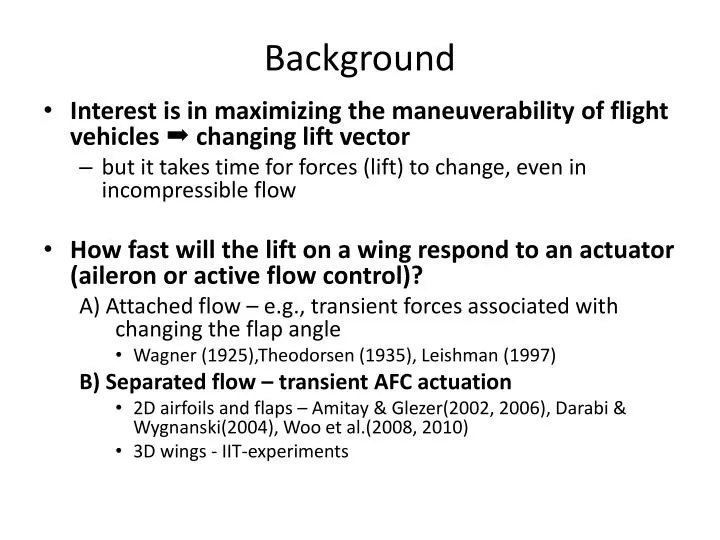
B ackground. Interest is in maximizing the maneuverability of flight vehicles changing lift vector but it takes time for forces (lift) to change, even in incompressible flow How fast will the lift on a wing respond to an actuator (aileron or active flow control)?

E N D
Background • Interest is in maximizing the maneuverability of flight vehicles changing lift vector • but it takes time for forces (lift) to change, even in incompressible flow • How fast will the lift on a wing respond to an actuator (aileron or active flow control)? A) Attached flow – e.g., transient forces associated with changing the flap angle • Wagner (1925),Theodorsen (1935), Leishman (1997) B) Separated flow – transient AFC actuation • 2D airfoils and flaps – Amitay & Glezer(2002, 2006), Darabi & Wygnanski(2004), Woo et al.(2008, 2010) • 3D wings - IIT-experiments
Summary of main points • Quasi-steady approach to flow control limited to very low frequencies – to increase bandwidth Active Flow Control (AFC) in unsteady flows requires • models for the unsteady aerodynamics • and the flow response to actuation • Both 2-D and 3-D Separated flows demonstrate time delays or lift reversals (RHP-zeros) in response to actuation • Response scales with the convective time and dynamic pressure • Lift reversals are connected with the LEV vortex formation and convection over the wing surface • Bandwidth limitations in closed loop control are set by fluid dynamic time delays, hence • Actuator performance characteristics can be determined • Different control architectures may be needed to achieve faster control, such as, predictive controllers
Outline of presentation • Active Flow Control in Unsteady Flows • Example Application: ‘gust’ suppression in unsteady freestream • Experimental set up, models, actuators • Steady state lift response • Quasi-steady and ad-hoc phase matching controller • Requirements for high(er)-bandwidth control • Unsteady aerodynamics model • Dynamic response to actuation • Robust controllers • CL-based • L-based • Role of time delays & rhp zeros • Useful for actuator design
Example application of AFC: u’-gust, L’ suppression Use AFC to suppress L’. Compare the performance of different control architectures Time varying flow conditions will require time-varying AFC
Unsteady flow wind tunnel & 2 wings • 6 component force balance – ATI Nano-17 • Shutters at downstream end of test section produce longitudinal flow oscillations – 0.10Uo • dSPACE® Real-Time-Hardware and software • Semi-circular planform (AR=2.54) • Angle of attack fixed at α=19o-20o • Wing I - 16 Micro-Valves Pulsed at 29Hz (St=0.84) – t63% const = 2.2 tconv • Wing II - piezoelectric actuators - t63%const= 0.2 tconv
Response to continuous actuation Continuous forcing at 29Hz pjet=34.5kPaCL=1.2 Uncontrolled flow – CL=0.75
Steady state lift curves & dominant lift/wake frequencies • Continuous pulsing at 29 Hz produced largest lift increment (StF-J = 0.4) With ‘dynamic’ AFC we are working between these two states.
Steady state lift response to actuator supply pressure Static lift coefficient map dependence on = 20of = 29 Hz St=1.2 Build a controller based on quasi-steady fluid dynamics Actuation range
Control architectures • Quasi-steady • Feed forward controller • Ad-hoc time delay and gain matching controller • Feed forward compensates for unsteady aero • Berlin robust control approach • CL tracking, robust feedback control • No unsteady aerodynamics model • L’ disturbance rejection, robust feedback control • Includes unsteady aerodynamics model • Comparison of slow and fast actuators
Valve control CL’ U∞ From hotwire FF controller SCW Plant Lift Quasi-steady feed-forward control • Assume • Subtract mean lift • Find CL’ for L’ = 0 => Actuator duty cycle controls CL’ • Required CL’
-10 dB Quasi-steady control L’ suppression Effective only at low frequencies, k<0.03, because model does not account for plant dynamics and unsteady aerodynamic effects
dφ/df dφ/dk Lift phase response to actuation frequency steady flow, = 20o td_3m/s = .35 s td_5m/s = .24 s + = td/tconv=5.8±0.5 5m/s 3m/s
Ad-hoc phase & gain matching Single point, feed forward control with harmonic freestream oscillation Compensate for time delays: 1) between lift response and actuation 2) between lift response and unsteady flow Increased controller speed 5x (k=0.15), but not the bandwidth Only works at a specific frequency
Requirements for high-bandwidth control • A model of the unsteady aerodynamic effects on the instantaneous lift • Amodel of the dynamic response of the wing to actuation (plant) • Pulse response provides insight into flow physics • Black-box models obtained using pseudo-random binary inputs and prediction error method of system identification
Pulse response is ‘common’ to many flows scales with t+ =tU/c, uj /U Max increment at t+=3 saturation Pulsed combustion actuator - Woo, et al. (2008) - 2D airfoil Pulsed-jet actuator – Kerstens, et al. (2010) – 3D wing Synthetic jet actuator – Quach, et al. (2010) See also: 2D Flap, Darabi & Wygnanski (JFM 2004) 2D Airfoil, Amitay & Glezer (2002, 2006) 3D Wing, Bres, Williams, & Colonius (APS-2010)
Flow behind the time delay ΔCLmin A B • Vien’spiv movie C ΔCLmax
System Identification used to obtain a model of the dynamic response of the wing Randomized step input experiments • Fixed supply pressure ( ), time intervals between step changes varied • Vary the flow speed • Vary the supply pressure Prediction error method of system identification • Measurements repeated at different supply pressures and different flow speeds to obtain 33 models • Averaged the models to obtain a 1st order (PT1) nominal model of the flow system, Gn(s)
Example of pseudo-random input data • used to obtain a ‘black box’ model of the wing’s lift response Input to actuator, Cpj0.5 Output ΔCL response
Bode plots and nominal system model • Input = Cpj0.5 Output = CL • PEM and pseudo-random square wave inputs used to obtain 33 models • Nominal first order model obtained from an average of family of models Nominal model Gn(s) is used to design both the feed forward and the feedback controllers
Control architectures • Quasi-steady • Feed forward controller • Ad-hoc time delay and gain matching controller • Feed forward compensates for unsteady aero • ‘Berlin’ robust control approach • CL tracking, robust feedback control • No unsteady aerodynamics model • L’ disturbance rejection, robust feedback control • Includes unsteady aerodynamics model • Comparison of slow and fast actuators
Predicted, u* (Cpj)0.5 Plant F(s) K(s) x (1/2ρU(t)2)S CL-based controller for U’-gust suppression Feed Forward Path Kff=F(s)Gn(s)-1 y = CL L f-1(u*) Lref r = CLref(t) H∞ Pre-compensator (squared input) (1/2ρU(t)2)S Hot-wire measurement of unsteady freestream converts Lref to CLref CL Feedback Path
Lift coefficient closed loop control Better performance than quasi-steady, but still only effective at low frequencies, k<0.04, Capable of suppressing “random” gusts (not only harmonics) Robust closed loop control of CL
Unsteady aerodynamic effects Frequency Response Measurements Lifts leads velocity in steady state sinusoidal forcing Lift lags the fluid acceleration Lift amplitude increases with increasing frequency Dynamic stall vortices formed during deceleration of flow
Lift-based controller for U’-gust suppression Hot wire measurement d = U’ Kd(s) Gd(s) Force balance measurement r = Lref y = L - K(s) G(s) u = pj - GD– Unsteady aerodynamic (disturbance) model KD – Feedforward disturbance compensation Gn – Pressure actuation model K – H∞controller to correct for uncertainties/errors in modeling Williams, et al. (AFC-II Berlin 2010), Kerstens, et al. AIAA -2010-4969 (Chicago 2010)
Dynamic response to pulsed-blowing actuation • Prediction-Error-Method used to model dynamic response to actuation • First order models with delay fit the measured data better than PT1 θ=0.157s
Bode plots of models at different flow speeds and actuator amplitudes • A nominal model is constructed from a family of 11 models at 7m/s • All-pass approximation causes deviations in phase at higher frequencies
Closed loop control bandwidth limitations • Time delays in the plant consist of: • Actuator delays • i-p regulator, plenum, plumbing for the pulsed-blowing actuator • Modulated pulse of the piezo-actuator • Time delay in the flow response to actuation • LEV formation and convection • For an ideal controller (ISE optimal) Skogestad& Postlethwaite (2005) • with time delay e-θs, the bandwidth is limited to ωc<1/θ. • θ=0.157s for pulsed blowing wing, fc < 1.0 Hz • with RHP real zero, for |S|<2 ωB<0.5z • Z=19.2 for piezo-actuator wing, fB< 1.5 Hz
Fast & slow actuators-step response Hot-wire measurement of actuator jet velocity • Piezo-actuator rise time is 10X faster than pulsed-blowing actuator. • Pulsed-blowing actuator has ‘plumbing’ delay • Faster actuators show initial lift reversal (non-minimum phase behavior) Lift/Lmax
Sensitivity functions Pulsed-blowing Actuator Uncontrolled plant – blue line Feedback only – green line Feedback and feedforward – red line Amplification of lift fluctuations Suppression of lift fluctuations • Sensitivity function shows disturbances will be amplified in the range of frequencies between ~0.9Hz to ~4.5Hz • Bandwidth is comparable for both actuators Piezo- Actuator
Pulsed-blowing control is effective with bandwidth of about 1.0 Hz, k=0.15 • Simulation results obtained using experimentally measured velocity and reference lift
Piezo-Actuator Control is Effective, with bandwidth about 0.9 Hz, k = 0.13 • Simulation results obtained using experimentally measured velocity and reference lift
Lift suppression spectra Pulsed Blowing Actuator Bandwidth is comparable for slow and fast actuators, because fluid dynamic time delays limit controller performance. Amplification of lift fluctuations Piezo-Actuator Suppression of lift fluctuations
Conclusions • Quasi-steady approach to flow control limited to very low frequencies - to increase bandwidth Active Flow Control (AFC) in unsteady flows requires models for the unsteady aerodynamics and the flow response to actuation • Controller bandwidth improvement was significant when the unsteady aero model was included • Both 2-D and 3-D Separated flows demonstrate time delays or lift reversals (RHP-zeros) in response to actuation • Response scales with the convective time and dynamic pressure • Lift reversals are connected with the LEV vortex formation and convection over the wing surface • Bandwidth limitations in closed loop control are set by fluid dynamic time delays, hence • Actuator design guidelines • Bandwidth ≈ ωc =1/θ or ωB=z/2 - higher bandwidth has little effect • Rise time < 1.5 c/U0 – faster rise time produces same lift response • Amplitude ≈ Ujet ≥ 2U0 – lift increment saturates