Download
1 / 16
160 likes | 381 Views
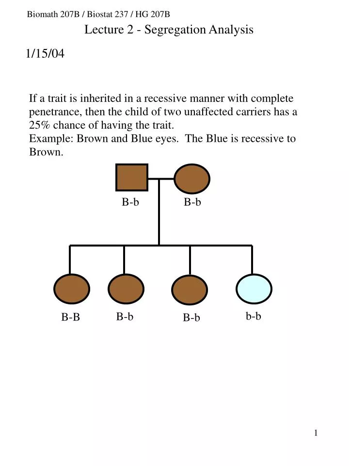
B-b. B-b. b-b. B-b. B-B. B-b. Biomath 207B / Biostat 237 / HG 207B. Lecture 2 - Segregation Analysis. 1/15/04. B-b. b-b. B-b. b-b. b-b. B-b. Simple segregation patterns: (1) recessive pattern of inheritance. (2) disease is fully penetrant (3) let D denote the disease allele

E N D
B-b B-b b-b B-b B-B B-b Biomath 207B / Biostat 237 / HG 207B Lecture 2 - Segregation Analysis 1/15/04
B-b b-b B-b b-b b-b B-b
Simple segregation patterns: (1) recessive pattern of inheritance. (2) disease is fully penetrant (3) let D denote the disease allele (4) p(d)=0.7, p(D)=0.3 (5) collect all families with exactly two children What distribution of affecteds do we expect to see under Hardy Weinberg Equilibrium and random mating? 75.1% 6.6% 1.1% Unaffected parents: 10.7% 1.9% 3.8% One affected parent (male or female): 0.8% Two affected parents:
A disease that is inherited in a dominant manner has a different pattern (1) disease is fully penetrant (2) let D denote the disease allele (3) p(d)=0.9, p(D)=0.1 (4) collect all families with exactly two children (5) Hardy Weinberg equilibrium and random mating 65.6% Unaffected parents: 7.3% 8.9% 14.6% One affected parent (male or female): 1.2% 0.2% 2.2% Two affected parents:
Why is it not always this simple? • More than one gene can be involved • and environment influences disease risk. That is, there are diseases with reduced penetrance and sporadic cases of disease. • Can’t sample everyone. Complete ascertainment is impractical for rare diseases • Family structures will vary. Parents may not be available.
Segregation Analysis • Goal of Segregation analysis: To identify the specific genetic mechanisms that may control traits associated with disease. • Segregation Analysis is used to determine if the observed familial aggregation has a genetic basis. In addition, it is used to estimate the relative effects of genetic and environmental factors shared among family members. It can also be used to test for gene-environmental interactions. • See Jarvik (1998) Complex Segregation analyses: Uses and Limitations AJHG 63:942-946 for more information.
Why go to all the trouble of segregation analysis? (1) Calculating relative risks isn’t good enough. Familial aggregation can be due to shared environment. High sibling relative risk (ls) or heritability does not prove that the disease has a genetic component (see for example, Guo AJHG 1998). Segregation analysis increases the confidence that genes play a role in the susceptibility to the disease. (2) The most powerful forms of linkage analysis require accurate knowledge of the inheritance mode and penetrance of the disease. Genetic model based gene mapping (classical linkage analysis) requires that the inheritance mode (dominant, recessive, etc) for the major gene and the probability of disease given a particular genotype be known. If the genetic model is wrong the false negative rate is increased (Martinez M. et al, Gen. Epi., 1989, 6:253-8).
The overall approach to segregation analysis is: • Step (1): Specify null and alternative hypotheses. • For example: no aggregation in families at all (sporadic model) for the null hypothesis and Mendelian inheritance (single gene) as the alternative hypothesis. • Step (2): Translate into mathematical models. • Step (3): Compute the maximum likelihood of the data and maximum likelihood estimates for the parameters in the mathematical model for both hypotheses. • Step (4): If the null model is a special case of the alternative (nested models), then compare the models using Likelihood ratio tests (LRT) to find the hypothesis that is best supported by the data (hierarchical testing). If not nested, then use AIC criterion or simulation to test. • Repeat these steps for as many hypotheses as you wish to test.
Comparing models: (1) If the null hypothesis is a special case of the alternative model then one way to compare is using a LRT test. For example a dominant Mendelian model is a restriction of the co-dominant Mendelian model. Under this null hypothesis: 2*LR has a chi-square distribution. The degrees of freedom are determined by the difference in the number of parameters. When comparing the dominant and codominant Mendelian models, the degree of freedom is one. The chi-square statistic has an associated p-value. If it is less than 0.05 then reject the null hypothesis in favor of the alternative. If it is greater than 0.05 then accept the null hypothesis. (2) If the null hypothesis is not a special case of the alternative use the AIC criterion to compare. For example, a dominant Mendelian model under HWE is not a special case of a recessive Mendelian model where we do not assume HWE. The model with the lowest AIC corresponds to the accepted hypothesis.
Converting hypotheses into models: • The mathematical models have three parts: • The penetrance – a measure of how likely is the trait value given a person is in a particular risk group In genetics, the most relevant parameters are m=gaa, gAa, gAA, representing the value for phenotype value for the aa, and the change in value for the Aa, or AA group. • The prior - The probability that a founder belongs to a particular risk group (under HWE determined by qA). • The transmission probabilities - The probability that an offspring belongs to a particular risk group given their parents’ risk groups. The relevant parameters taa, tAa, and tAA. For example taa = P(A transmitted from an aa parent) and taataa =P(AA transmitted from aa and aa parents) Under Mendelian inheritance, taa= 0, tAa=1/2, and tAA=1.