Download
1 / 32
320 likes | 647 Views
Multilevel Graph Partitioning and Fiduccia-Mattheyses. Wasim Mohiuddin. Papers. A Fast and High Quality Multilevel Scheme for Partitioning Irregular Graphs, 1995 A Coarse-Grain Parallel Formulation of Multilevel k-way Graph Partitioning Algorithm, 1997 Authors: George Karypis and Vipin Kumar

E N D
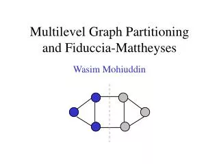
Multilevel Graph Partitioning and Fiduccia-Mattheyses Wasim Mohiuddin
Papers • A Fast and High Quality Multilevel Scheme for Partitioning Irregular Graphs, 1995 • A Coarse-Grain Parallel Formulation of Multilevel k-way Graph Partitioning Algorithm, 1997 • Authors: George Karypis and Vipin Kumar • Link: www.cs.umn.edu/~metis
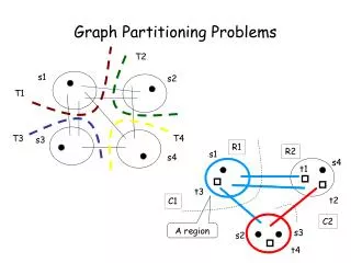
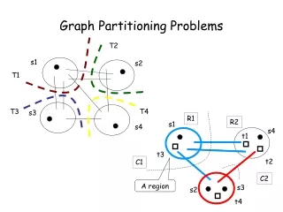
Applications • Graph partitioning is an important problem that has extensive applications in many areas: • Scientific Computing • VLSI Design • Task Scheduling
Parallel Algorithms and Graphs • The implementation of many parallel algorithms require solutions graph partitioning problems • Vertices represent computational tasks • Edges represent data exchanges • Vertices and Edges can be assigned weights proportional to the amount of work involved
Vertices are assigned a weight proportional to their task • Edges are assigned weights that reflect the amount of data that needs to be exchanged
Graph Partitioning • NP-complete • Many algorithms have been developed that find reasonably good partitions: • Spectral Partitioning • Geometric Partitioning • Multilevel Graph Partitioning
Multilevel Graph Partitioning • 3 Phases • Coarsen • Partition • Uncoarsen
Multilevel Graph Partitioning • Phase 1 • Coarsen • Partition • Uncoarsen
Coarsening Phase • A coarser graph can be obtained by collapsing adjacent vertices • Matching, Maximal Matching • Different Ways to Coarsen • Random Matching (RM) • Heavy Edge Matching (HEM) • Light Edge Matching (LEM) • Heavy Clique Matching (HCM)
Multilevel Graph Partitioning • Phase 2 • Coarsen • Partition • Uncoarsen
Partitioning Phase • The second phase of a multilevel algorithm computes a high-quality (i.e., small edge-cut) Pm of the coarse graph Gm = (Vm, Em) such that each part contains roughly half of the vertex weight of the original graph.
Partitioning Algorithms • Spectral Bisection (SB) • Kernighan-Lin (KL) • Fiduccia-Mattheyses (FM) • Graph Growing Algorithm (GGP) • Greedy Graph Growing Algorithm (GGGP)
Kernighan-Lin Algorithm • Iterative in nature • Starts with an intial bipartition of the graph • In each iteration, it searches for a subset of vertices from each part of the graph such that swapping them leads to a partition with a smaller edge-cut • Each iteration takes O(E log E)
Fiduccia-Mattheyses Algorithm • An improvement on the original KL algorithm • Reduces complexity to O(E) by using appropriate data structures
Simplified Fiduccia-Mattheyses: Example (1) 1 0 a b Grey nodes are in Part1; Black nodes are in Part2. The initial partition into two parts is arbitrary. In this case it cuts 8 edges. The initial node gains are shown in Grey. -1 1 0 2 c d f e g h 0 3 Nodes tentatively moved (and cut size after each pair): none (8);
Simplified Fiduccia-Mattheyses: Example (2) 1 0 a b The node in Part1 with largest gain is g. We tentatively move it to Part2 and recompute the gains of its neighbors. Tentatively moved nodes are hollow circles. After a node is tentatively moved its gain doesn’t matter any more. -3 1 -2 2 c d f e g h -2 Nodes tentatively moved (and cut size after each pair): none (8); g,
Simplified Fiduccia-Mattheyses: Example (3) -1 -2 a b The node in Part2 with largest gain is d. We tentatively move it to Part1 and recompute the gains of its neighbors. After this first tentative swap, the cut size is 4. -1 -2 0 c d f e g h 0 Nodes tentatively moved (and cut size after each pair): none (8); g, d (4);
Simplified Fiduccia-Mattheyses: Example (4) -1 -2 a b The unmoved node in Part1 with largest gain is f. We tentatively move it to Part2 and recompute the gains of its neighbors. -1 -2 c d f e g h -2 Nodes tentatively moved (and cut size after each pair): none (8); g, d (4); f
Simplified Fiduccia-Mattheyses: Example (5) -3 -2 a b The unmoved node in Part2 with largest gain is c. We tentatively move it to Part1 and recompute the gains of its neighbors. After this tentative swap, the cut size is 5. 0 c d f e g h 0 Nodes tentatively moved (and cut size after each pair): none (8); g, d (4); f, c (5);
Simplified Fiduccia-Mattheyses: Example (6) -1 a b The unmoved node in Part1 with largest gain is b. We tentatively move it to Part2 and recompute the gains of its neighbors. 0 c d f e g h 0 Nodes tentatively moved (and cut size after each pair): none (8); g, d (4); f, c (5); b
Simplified Fiduccia-Mattheyses: Example (7) -1 a b There is a tie for largest gain between the two unmoved nodes in Part2. We choose one (say e) and tentatively move it to Part1. It has no unmoved neighbors so no gains are recomputed. After this tentative swap the cut size is 7. c d f e g h 0 Nodes tentatively moved (and cut size after each pair): none (8); g, d (4); f, c (5); b, e (7);
Simplified Fiduccia-Mattheyses: Example (8) a b The unmoved node in Part1 with the largest gain (the only one) is a. We tentatively move it to Part2. It has no unmoved neighbors so no gains are recomputed. c d f e g h 0 Nodes tentatively moved (and cut size after each pair): none (8); g, d (4); f, c (5); b, e (7); a
Simplified Fiduccia-Mattheyses: Example (9) a b The unmoved node in Part2 with the largest gain (the only one) is h. We tentatively move it to Part1. The cut size after the final tentative swap is 8, the same as it was before any tentative moves. c d f e g h Nodes tentatively moved (and cut size after each pair): none (8); g, d (4); f, c (5); b, e (7); a, h (8)
Simplified Fiduccia-Mattheyses: Example (10) a b After every node has been tentatively moved, we look back at the sequence and see that the smallest cut was 4, after swapping g and d. We make that swap permanent and undo all the later tentative swaps. This is the end of the first improvement step. c d f e g h Nodes tentatively moved (and cut size after each pair): none (8); g, d (4); f, c (5); b, e (7); a, h (8)
Simplified Fiduccia-Mattheyses: Example (11) a b Now we recompute the gains and do another improvement step starting from the new size-4 cut. The details are not shown. The second improvement step doesn’t change the cut size, so the algorithm ends with a cut of size 4. In general, we keep doing improvement steps as long as the cut size keeps getting smaller. c d f e g h
Multilevel Graph Partitioning • Phase 3 • Coarsen • Partition • Uncoarsen
Uncoarsening Phase • During the uncoarsening phase, the partitioning of the coarser graph Gmis projected back to the original graph by going through the graphs Gm-1,Gm-2,…,G1. • Since each vertex u in Vi+1 contains a distinct subset U of vertices of Vi, the projection of the partition from Gi+1 to Giis constructed by simply assigning the vertices in U to the same partition in Githat vertex u belongs in Gi+1.
Multilevel Graph Partitioning and Fiduccia-Mattheyses Thank You Questions?