Download
1 / 43
430 likes | 444 Views
Graph Partitioning. Abhiram Ranade IIT Bombay. A load balancing problem. Input: undirected graph G. Vertices = processes. Edges = interprocess communication. integer k = number of available processors. Output: Assign processes to processors. , 4. A load balancing problem. Input:

E N D
Graph Partitioning Abhiram Ranade IIT Bombay
A load balancing problem • Input: • undirected graph G. Vertices = processes. Edges = interprocess communication. • integer k = number of available processors. • Output: Assign processes to processors , 4
A load balancing problem • Input: • undirected graph G. Vertices = processes. Edges = interprocess communication. • integer k = number of available processors. • Output: Assign processes to processors Give equal number of processes to each processor. Minimize actual communication , 4
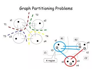
The graph partitioning problem • Input: undirected graph G, integer k • Output: Partition into subgraphs G1, G2, …, Gk with equal number of vertices, by removing minimum number of edges. , 2 , 3
The graph partitioning problem • Input: undirected graph G, integer k • Output: Partition into subgraphs G1, G2, …, Gk with equal number of vertices, by removing minimum number of edges. , 2 , 3
Other motivations • Divide and conquer algorithms on graphs. • Partition into balanced subgraphs. • Recurse on subgraphs. • Cost of combine step : high if large number of edges between subgraphs. • Identify bottlenecks in graph for purpose of fault tolerance etc. • Nice connections to geomtry.
Outline • Basic results • Partitioning special classes of graphs • Planar graphs • FEM (finite element method) graphs • Partitioning arbitrary graphs • Spectral Methods • More advanced methods • Heuristics
Some basic results • NP-hard even for k=2. • Reduction from MAX-CUT. • Polytime algorithm known for trees • Moderately hard exercise. Dynamic programming • Other graph classes: next • Approximation algorithm: O(log1.5n) factor known. • intro to some of the ideas: later
Planar graphs • NP-complete? Not known. • Lipton-Tarjan Planar Separator Algorithm: • Any planar graph with n vertices can be bisected by removing O(√n) vertices and incident edges. • O(√n) edges for bounded degree graphs. • Algorithm may give O(√n) separator even if smaller exists. • Optimal for “Natural planar graphs” which cannot be bisected without removing Ω(√n) vertices.
Planar separator theorem • Every planar graph can be bisected by removing O(√n) vertices. • Lipton-Tarjan proof: • uses clever breadth first search. • Today: Alternate proof • Elegant connection to geometry. Extends to other geometrically embedded graphs, e.g. FEM graphs.
Representing planar graphs by “kissing” disks http://isabelandbenson.wordpress.com/2012/02/12/a-planar-separation-proof-using-koebes-theorem/
Circle packing theorem Theorem [Koebe 1936] For every planar graph with n vertices, there exist disjoint circles c1, c2, …, cn such that ci and cj are tangential iff vi, vj are connected by an edge. …Kissing disk embedding
Circle packing example (Wikipedia)
Algorithm to find a Planar Separator • Get a kissing disk embedding. • Stereographically project it onto a sphere. • Find “center point” of disk centers. • Adjust so that center point moves to sphere center • Separator = random great circle through center. Theorem: Each hemisphere has θ(n) vertices. Expected number of edges cut = O(√n).
Remark • Algorithm may not produce exact bisection, but say, ¼, ¾ split of vertices. • Repeat on larger partition if balance not achieved. ¾ splits into 9/16, 3/16 • Combine ¼ + 3/16 = 7/16. • Now we have better balance: 7/16, 9/16. • Repeating log times suffices. Number of edges cut increase only by constant factor.
Stereographic projection Input: Disk embedding on horizontal plane. • Place a sphere on the plane. • Point P’ on plane mapped to P on sphere such that PP’ passes through North Pole. • Circles map to circles! (Wikipedia)
Algorithm to find a Planar Separator • Get a kissing disk embedding. ✓ • Stereographically project it onto a sphere. ✓ • Find “center point” of disk centers. • Adjust so that center point moves to sphere center • Separator = random great circle through center.
Centerpoint C of n points C = point such that any plane through it has at least n/4 points on both sides. • Centerpoints exist, and may not be unique. • Approximate centerpoints are easily found. Will guarantee at least n/Q points on both sides, where Q maybe > 4.
Algorithm to find a Planar Separator • Get a kissing disk embedding. ✓ • Stereographically project it onto a sphere. ✓ • Find “center point” of disk centers. ✓ • Adjust so that center point moves to sphere center • Separator = random great circle through center.
Adjusting the centerpoint Centerpoint shown in red. Project back onto inclined plane. Use a bigger sphere having same point of contact. How does red point move?
Where are we? • We have a sphere with a disk on it for each vertex. • Disks touch if corresponding vertices have an edge. • Center of sphere = centerpoint of vertices. • What will happen if we partition using some great circle? • Centerpoint: θ(n) vertices will be on each side • Will too many disks intersect with great circle?
How many disks intersect with a random great circle? • Pick a random great circle = pick a random point as its north pole. • Probability = Band area/sphere area = 2r*2πR/4πR2 = r/R disk of radius r R = sphere radius Band in which north pole should lie to intersect with disk.
Expected number of intersections • E = r1/R + r2/R + … rn/R • We know: πr12 + πr22 + … + πrn2 ≤ 4πR2 • E is maximized when all ri are equal, ri ≤ 2R/√n • E ≤ n * (2R/√n)/R = 2√n • Plane has at least n/4 vertices on each side • By removing incident edges on √n vertices we get ¼ - ¾ partition of vertices. • Clearly such a partition exists! QED!
Remarks • Nice connection between graph theory and geometry. • Great circle when projected back, becomes a circle on the graph. “Circle separator” • Do we need circles? Can we hope to get good partitions using a straight line? • There exist graphs for which this is not possible. • In practice, Lipton-Tarjan’s original algorithm will be faster than above algorithm.
Finite Element Method (FEM) Graphs http://www.geuz.org/gmsh/gallery/bike.png
FEM Graphs • 3 dimensional object represented by collection of volumes, “elements” • Element size: • Small where physical properties vary a lot. • Large where physical properties vary less. • “Aspect ratio” of elements is small, i.e. elements are not flat/narrow. • Useful for to reduce floating point overflow..
FEM Graphs continued • Effectively we have a “kissing disk” embedding of elements in 3 dimensional space. • Theorem[Miller-Thurston 1990] A 3d FEM mesh with n elements of small aspect ratio can be bisected by removing O(n2/3) edges. • Partitioning FEM graphs is useful for load balancing on parallel computers.
Partitioning General Graphs V - S • Don’t insist on bisection. • Sparsity = |C|/|S| • Cut ratio = |C|/(|S||V-S|) • Sparsity/C.Ratio ≈ |V| • We study algorithms that attempt to find cuts of minimum ratio. • We can get bisection by repeating if necessary. S C
Strategy Our optimization problem is expressed in the language of graphs. • Pose it as a problem on integer variables. • NP-complete. • Find a similar problem on real variables that can be solved in polynomial time. • Exploiting the symmetry, get back an integer solution. Hope: it is close to the optimal.
Algebraic definition of cut ratio • x = bit vector. xi = 1 iff ith vertex is in S. • No. of crossing edges: • |S||V-S| = • Want to minimize V-S S 1 3 4 2
General Algorithmic Strategy: Relaxation • Problem 1: minimize 3x2 - 5x, x is an integer. • Problem 2: minimize 3x2 - 5x, x is real. - Easier to solve, make derivative = 0 etc. - min(Problem 1) ≥ min(Problem 2) • Problem 2 = Relaxation of problem 1 • Strategy to solve problem 1: solve problem 2 and then take a nearby solution. • Minimizing cut ratio: similar idea..
Relaxation to “solve” for cut ratio • Want to find • Allow real values • Suppose we can solve for x. • We will “round” solution • high = 1. Low = 0. • Insist that xi add to 1
contd. Lij = -1 if (i,j) is an edge, = degree(i) if i=j, =0 otherwise L = “Laplacian of the graph” σ2 is second smallest “Eigenvalue of L” Can be calculated quickly. minimizing x can also be calculated.
Algorithm for finding good ratio cut • Construct Laplacian matrix • Find second smallest eigenvector • Choose threshold t. • Partition = {i | xi ≤ t}, {i | xi > t} How to choose t? Try all possible choices, and take one having best ratio. “Spectral Method” : eigenvectors involved.
How good is the partition • Cheeger’s Theorem: • Partition found by previous algorithm will have cut ratio at most Difficult proof • Optimal partition will have cut ratio at least Just proved! • Seems to work well in practice
Examples • Cycle on n vertices: Spectral method finds optimal partition. • Bounded degree planar graphs: Spectral method finds O(√n) sized bisector. • Binary hypercube: Spectral methods will find cut of ratio √4logn / n, whereas opt ratio = 1/n
Remarks about intuition • How did we steer the analysis towards the Laplacian? • Experience • Laplacian arises in solving differential equation, where second eigenvalue gives how graph may “vibrate”. Vibration mode points to cuts. • Laplacian is related to SVD, singular value decomposition. SVD of a point cloud identifies length, breadth, width of cloud. Small cuts are perpendicular to length.
Advanced methods • Starting point: • Different ways to relax. • If you relax too much, you may be able to solve the new problem more easily, but the solution will be too far. • Arora-Rao-Vazirani 04 : stricter relaxation. Always give cut with ratio = O(√log n) times optimal.
Heuristics • Graph coarsening [Metis 04]: • Pick disjoint edges in graph. • Merge endpoints of each edge into a single vertex. (fast) • Repeat several times. • Find partition for final “coarse” graph using sophisticated method. (slow, but on small graph) • Final partition induces partition on original graph.
Concluding Remarks • Important problem • Many applications • Many interesting methods. Theory + Heuristic. • Deep connections to geometry.
Generalization of bisection • We may need to cut many edges to bisect, but by cutting very few we may get ¼ - ¾ split. • May be useful to know such “bottlenecks” • Even for bisection, it might be easier to get one piece at a time
c-balanced partitioning • For a fixed c, remove as few edges as possible to get subgraphs of size cn, (1-c)n. • If c=O(1), we can use repeatedly to achieve bisection. Example: c = 0.1 • After 1 application we have 0.1 – 0.9 split. • Apply once more on 0.9 : 0.1, 0.09, 0.81 • Apply log times on larger piece and extract n/2 vertices. Bisection!