Graph Partitioning in Parallel

1. Graph Partitioning in Parallel Jordan Denny & Mike Froning

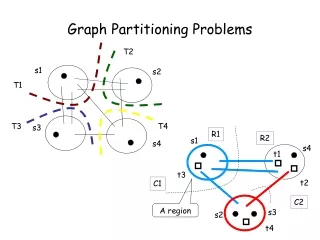
2. What is Graph Partitioning? • Graph partitioning involves partitioning a graph G = (V,E) into two (or more) sub graphs • V represents the set of vertices in the graph • E represents the set of edges in the graph • An edge connects two vertices together • The goal of graph partitioning is to partition a graph G into two (or more) sub graphs, S1, S2, … Sn, such that the edges between each sub graph is minimized

3. Balanced Graph Partitioning • Also known as Uniform Graph Partitioning • This is a subset of the Graph Partitioning problem where the goal is to both minimize the edges between sub graphs and keep the size of each sub graph the same • Some graph partitioning algorithms are only concerned with keeping the edges minimized, others attempt to keep the sub graphs balanced • The Balanced Graph Partitioning problem can be formulated using what’s known as the Cut Ratio

4. Cut Ratio • The cut ratio will be defined as • The cut ratio is defined as the number of edges between each of the resulting sub graphs divided by the number of vertices in the smallest of the resulting sub graphs • The goal of balanced graph partitioning is to minimize the cut ratio • The best partition is the one with the fewest edges between sub graphs with each sub graph having an equal number of vertices

5. Difficulties • Graph partitioning is an NP-Complete problem • Any solution is based on heuristics • There are a large number of different graph partitioning algorithms out there • Each one has its pros and cons • Some sacrifice speed for improved quality, others sacrifice quality for improved speed

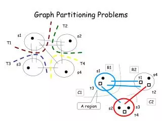
6. Sample Graph • G = (V,E) • E = {(1,2),(1,3),(2,4),(3,4),(3,5),(4,6),(5,6),(5,7),(6,8),(7,8)} |E| = 10 • V = {1, 2, 3, 4, 5, 6, 7, 8} |V| = 8

7. Example • e(S1,S2)= {(3,5),(4,6)} |e(S1,S2)| = 2 • This is the best possible partition for this graph

8. Applications • There are many different applications for graph partitioning, including: • Scientific Computing • The vertices of the graph model computations • The edges model dependencies among these computations • The graph needs to be partitioned such that dependencies across different processors are minimized • VLSI Circuit Design • Find the minimal number of clusters of vertices inside of a design • This will allow a smaller amount of interconnections and cuts in a design, which will allow for a smaller area and/or fewer chips

9. Applications • Task Scheduling • If V = {tasks}, each unit cost, an edge e=(i,j) means task i has to communicate with task j • Then partitioning means balancing the load and minimizing communication volume • Image Segmentation • Image segmentation involves partitioning a digital image into multiple segments • Goal is to simplify the representation of the image into something easier to analyze • Using graph partitioning, the image is modeled as a weighted, undirected graph • Pixels are associated with vertices and edges have weights that define how similar neighboring vertices are • The graph is partitioned in order to model good clusters

10. Graph Partitioning Algorithms • Local vs. Global • Both categories are based on heuristics • Local methods involve picking a starting vertex and going through the graph one step at a time without any knowledge on the overall graph structure • Examples of local algorithms include Kernighan-Lin and Fiduccia-Mattheyses • Global methods rely on the overall structure of the graph and are not dependent upon choosing a good initial vertex • An example of a global algorithm is spectral partitioning

11. Four Algorithms • We will now discuss four different algorithms for graph partitioning, their time complexities, and how they can be parallelized • One is a local algorithm for partitioning a graph into two sub graphs that focuses on running time • One is a global algorithm for partitioning a graph into two sub graphs that focuses on running time • One is an algorithm that partitions a graph into k-sub graphs that focuses on running time • One is an algorithm that attempts to achieve the best possible partition of the graph

12. Kernighan-Lin Algorithm • Given an arbitrary initial partition of the graph G into two sub graphs S1 and S2, the Kernighan-Lin (KL) algorithm repeatedly improves the partition by performing several iterations, with each iteration improving the result, until a local optimum is reached • The idea behind KL is that, after the initial partition, there are a set of vertices in S1 and an equal number in S2 that are out of place • If these vertices were swapped between sub graphs, the partition would be optimal • The KL algorithm tries to find these out of place vertices

13. Kernighan-Lin Algorithm • A ‘D value’ is calculated for each vertex • This value is a measure of how out of place a vertex is • The ‘D value’ for vertex a would be calculated as • Where Ea is a measure of how strongly attracted vertex a is to S1 and Iais a measure of how strongly attracted vertex a is to S2 • Thus, the larger the ‘D value’ is for a particular vertex, the more likely that it should be in the sub graph S1 rather than S2

14. Kernighan-Lin Algorithm • Whenever you are considering a swap, you are looking at two vertices at a time, a and b • The calculation for Db is similar to that of Da • Once the D values are calculated, the gain for swapping the two vertices, gab, needs to be calculated where Cab is the number of edges between a and b

15. Kernighan-Lin Algorithm • The algorithm works by first computing D values for every vertex • Next, the algorithm considers every pair of vertices and determines the gain that would be achieved by swapping them • Once identified, these vertices are locked and cannot be considered again this iteration, and D values are updated • Once every vertex has been checked, the algorithm finds which swap results in the best improvement • The algorithm then swaps all of the vertices up to the one that produced the best improvement • This process continues until no more improvements can be made

16. Kernighan-Lin Algorithm Pseudocode

17. Parallelizing Kernighan-Lin • The sequential running time of the KL algorithm is O • This algorithm can be parallelized very easily • Step 1 can be parallelized by dedicating one processor to each vertex, and having each processor calculate the D value for its vertex • Step 2 can be parallelized by sorting the D values and parallelizing the computation of swapping gains • Step 3 can be parallelized with an MPI_Reduce (MPI_MAX) call • Step 4 can be parallelized with each processor swapping its vertex if needed and using an All-to-All broadcast • Tseq = O Tpar = O • Speedup = Efficiency =

18. Spectral Partitioning • Spectral partitioning is a global method for partitioning the graph • Let G = (V,E) be an undirected graph with |V| = n vertices • We let A = A(G) be an n x n adjacency matrix relevant to G with one row and one column for each vertex • au,v equals one if an edge exists between vertices u and v, zero otherwise • The matrix has 0s along the diagonal (no loops on the graph) and is symmetric (au,v = av,u)

19. Spectral Partitioning • We then define a Laplacian Matrix, L(G) • L(G) is an n x n symmetric matrix with one row and one column for each vertex • Li,i(G) = di = degree of vertex i • Lu,v(G) = -1 if an edge exists between vertices u and v • Lu,v(G) = 0 otherwise • The matrices L(G) and A(G) are related via L = D – A • with D being a diagonal matrix where di,i is the vertex degree of node i

20. Examples of A, L, and D (L = D – A)

21. Spectral Partitioning • The spectral partitioning algorithm is based on the intuition that the second lowest vibrational mode of a vibrating string naturally divides the string in half

22. Spectral Partitioning • Applying that intuition to the eigenvectors of a graph we obtain the partitioning • The lowest eigenvalue of the Laplacian matrix defined earlier is zero and the corresponding eigenvector provides no information about the graph structure • However, the second eigenvector, called the Fiedler Vector, can be used • Dividing its elements according to the median, we obtain two partitions • We can also use the third, fourth, or bigger eigenvector to obtain three, four or more partitions

23. Spectral Partitioning – The Algorithm Input: a graph G = (V, E) Output: two sub graphs S1= (V1, E1), S2= (V2, E2) 1. compute the Fiedler eigenvector v 2. search median of v 3. for each vertex i of G 3.1. if v(i) ≤ median put vertex i in partition V1 3.2. else put vertex i in partition V2 4. if |V1| − |V2| > 1 move some vertices with components equal to median from V1 to V2to make this difference at most one 5. let V1’ be the set of vertices in V1 adjacent to some vertex in V2 let V2’ be the set of vertices in V2 adjacent to some vertex in V1 set up the edge separator E’ = the set of edges of G with one point in V1’ and the second in V2’ 6. let E1 be the set of edges with both end vertices in V1 let E2 be the set of edges with both end vertices in V2 set up the graphs S1= (V1, E1), S2= (V2, E2) 7. end

24. Spectral Partitioning Time Complexity • The time intensive part of the algorithm involves computing the eigenvector • The QR algorithm is the standard method for computing the eigenvalues of a matrix • Sequentially, this takes O time • We can also use sequential “norm-reducing” algorithms that display quadratic convergence in most cases • A parallel form of the “norm-reducing” algorithm exists that can be implemented using processors • Using this algorithm, we can perform Spectral Partitioning in parallel in O time • Tseq = O Tpar = O • Speedup = Efficiency =

25. Recursive Bisection • How do we perform a k-way partition? • Idea is that it is easier to partition a graph into two sub graphs rather than k sub graphs in one step • Partition the graph into two sub graphs, partition each sub graph into two more sub graphs, and keep recursing into you get k sub graphs • Two advantages: • Each sub problem is easier than the general problem • Natural parallelism • First step is a sequential problem, two-way parallelism at the second step, four-way parallelism at the third step, etc. • Partitioning a graph into k sub graphs is achieved in logk steps

27. Recursive Bisection • Typically the graph is partitioned using a 2-way algorithm like Kernighan-Lin • However, because the 2-way graph partitioning problem is NP-Complete, practical Recursive Bisection algorithms use more efficient heuristics in place of an optimal bisection algorithm • Most such heuristics are designed to find the best possible bisection within allowed time • Some extended heuristics have been proposed that apply quadsection or octsection in place of bisection • Hendrickson and Leland have published results that quadsectioning or octsectioning, though more expensive then bisectioning, give the algorithm better quality

28. Evolutionary Algorithm • Evolutionary algorithms apply the principles of macroevolution to computer programming • EA’s are optimization algorithms; they attempt to find the optimal solution to a given problem • An evolutionary algorithm consists of 8 steps: • Representation of the problem • Creating a fitness function • Generating an initial population of individuals • Selecting the “best” individuals from that population to be parents • Mating those parents to produce offspring • Mutating those offspring into (hopefully) better offspring • Selecting the “best” individuals to survive and killing off the rest • Repeat steps 4-7 over and over until a termination criterion is reached

29. Evolutionary Algorithm Implementation • Representation – Bit strings (ex. 00001111) • Fitness function – Cut Ratio () • Initialization – Uniform Random • Parent Selection – Tournament without Replacement • Recombination – Uniform Crossover ex. 00001111 and 10101010 produces: 10101010 • Mutation – Bit flip ex. 10101010 becomes 10001010 • Survivor Selection – Tournament without Replacement • Termination – 100 Generations

30. Example: • B = 00001111 • The red colors represent sub graph 0, the blue colors represent sub graph 1

31. Example: • The fitness of B = 00001111 would be • A fitness value will be stored inside of every bit string, and that fitness will be used to determine which bit strings are better than others • A lower fitness value represents a better partition

32. Evolutionary Algorithm Time Complexity • For a graph with N vertices and an EA with population size E, S parents, C children, K tournament size • Sequential times: • Initialization – O(N*E) • Parent Selection – O(K*S) • Recombination – O(N*C) • Mutation – O(N*C) • Fitness evaluations – O) • Survivor Selection – O(E*K) • Obviously the most time intensive part of the algorithm is using the bit string to partition the graph • The graph is represented by an NxN matrix, and it takes roughly O() time to calculate the fitness of one individual

33. Parallelizing the Evolutionary Algorithm • Luckily, each step of the EA is easily parallelizable • If we have N processors, we can greatly speedup each step of the algorithm • Initialization – O(N*E) becomes O(logN*E) • Parent Selection – O(K*S) becomes O(logN*S) assuming K=N • Recombination – O(N*C) becomes O(logN*C) • Mutation – O(N*C) becomes O(logN*C) • Fitness evaluations – O(*C)becomes O(*logC) • Survivor Selection – O(E*K) becomes O(logN*S) assuming K=N • This means that the running time of a parallel Evolutionary Algorithm is roughly the same as a sequential graph partitioning algorithm • But, this is the time complexity for one generation, and we typically perform several generations in an Evolutionary Algorithm • However, using an Evolutionary Algorithm, we can achieve very good solutions in roughly the same time as the graph partitioning algorithms take by themselves

34. Conclusions • If no knowledge about the overall structure of the graph is known and you need solution quickly, use the Kernighan-Lin Algorithm • If the overall structure of the graph is known and you need a solution quickly, use Spectral Partitioning • If you need to partition the graph into more than two sub graphs, use Recursive Bisection • If you need a very good partition, use an Evolutionary Algorithm • These four algorithms are just a few of the many different strategies for partitioning a graph • Graph Partitioning is an NP-Complete problem • Graph Partitioning has a wide array of applications, and finding optimal strategies to partition a graph is of high importance to computer scientists

35. Sources • Parallel Methods for Vlsi Layout Designby Si. Pi Ravikumār • Introduction to Evolutionary Computing by A.E. Eiben and J.E. Smith • http://citeseerx.ist.psu.edu/viewdoc/summary?doi=10.1.1.134.3566 • http://citeseerx.ist.psu.edu/viewdoc/summary?doi=10.1.1.40.4680 • http://www.cc.gatech.edu/~bader/COURSES/GATECH/CSE-Algs-Fall2011/papers/KK95b.pdf • http://www.siam.org/meetings/csc11/monien.pdf • http://eda.ee.ucla.edu/EE201A-04Spring/mP.ppt • http://www.cs.berkeley.edu/~yelick/cs267_sp07/lectures/lecture25/lecture25_loadbal_ky07.ppt • http://www.cs.cmu.edu/~jshi/papers/pami_ncut.pdf • http://web.mst.edu/~ercal/387/slides/ • http://www.netlib.org/utk/lsi/pcwLSI/text/node253.html