Download
1 / 57
590 likes | 992 Views
Bivariate Analyses. Bivariate Procedures I Overview. Chi-square test T-test Correlation. Chi-Square Test. Relationships between nominal variables Types: 2x2 chi-square Gender by Political Party 2x3 chi-square Gender by Dosage (Hi vs. Med. Vs. Low). Starting Point: The Crosstab Table.

E N D
Bivariate Procedures I Overview • Chi-square test • T-test • Correlation
Chi-Square Test • Relationships between nominal variables • Types: • 2x2 chi-square • Gender by Political Party • 2x3 chi-square • Gender by Dosage (Hi vs. Med. Vs. Low)
Starting Point: The Crosstab Table • Example: Gender (IV) Males Females Democrat 1 20 Party (DV) Republican 10 2 Total 11 22
Column Percentages Gender (IV) Males Females Democrat 9% 91% Party (DV) Republican 91% 9% Total 100% 100%
Row Percentages Gender (IV) Males Females Total Democrat 5% 95% 100% Party (DV) Republican 83% 17% 100%
Full Crosstab Table Males Females Total Democrat 1 20 21 5% 95% 9% 91% 64% Republican 10 2 12 83% 17% 91% 9% 36% Total 11 22 33 33% 67% 100%
Research Question and Hypothesis • Research Question: • Is gender related to party affiliation? • Hypothesis: • Men are more likely than women to be Republicans • Null hypothesis: • There is no relation between gender and party
Testing the Hypothesis • Eyeballing the table: • Seems to be a relationship • Is it significant? • Or, could it be just a chance finding? • Logic: • Is the finding different enough from the null? • Chi-square answers this question • What factors would it take into account?
Factors Taken into Consideration • Factors: • 1. Magnitude of the difference • 2. Sample size • Biased coin example • Magnitude of difference: • 60% heads vs. 99% heads • Sample size: • 10 flips vs. 100 flips vs. 1 million flips
Chi-square • Chi-Square starts with the frequencies: • Compare observed frequencies with frequencies we expect under the null hypothesis
What would the Frequencies be if there was No Relationship? Males Females Total Democrat 21 Republican 12 Total 11 22 33
Expected Frequencies (Null) Males Females Total Democrat 7 14 21 Republican 4 8 12 Total 11 22 33
Comparing the Observed and Expected Cell Frequencies • Formula:
Calculating the Expected Frequency • Simple formula for expected cell frequencies • Row total x column total / Total N • 21 x 11 / 33 = 7 • 21 x 22 / 33 = 14 • 12 x 11 / 33 = 4 • 12 x 22 / 33 = 8
Observed and Expected Cell Frequencies Males Females Total Democrat 17 20 14 21 Republican 10 4 2 8 12 Total 11 22 33
Plugging into the Formula O - E Square Square/E Cell A = 1-7 = -6 36 36/7 = 5.1 Cell B = 20-14 = 6 36 36/14 = 2.6 Cell C = 10-4 = 6 36 36/4 = 9 Cell D = 2-8 = -6 36 36/8 = 4.5 Sum = 21.2 Chi-square = 21.2
Is the chi-square significant? • Significance of the chi-square: • Great differences between observed and expected lead to bigger chi-square • How big does it have to be for significance? • Depends on the “degrees of freedom” • Formula for degrees of freedom: (Rows – 1) x (Columns – 1)
Chi-square Degrees of Freedom • 2 x 2 chi-square = 1 • 3 x 3 = ? • 4 x 3 = ?
df P = 0.05 P = 0.01 P = 0.001 1 3.84 6.64 10.83 2 5.99 9.21 13.82 3 7.82 11.35 16.27 4 9.49 13.28 18.47 5 11.07 15.09 20.52 6 12.59 16.81 22.46 7 14.07 18.48 24.32 8 15.51 20.09 26.13 9 16.92 21.67 27.88 10 18.31 23.21 29.59 Chi-square Critical Values * If chi-square is > than critical value, relationship is significant
Multiple Chi-square • Exact same procedure as 2 variable X2 • Used for more than 2 variables • E.g., 2 x 2 x 2 X2 • Gender x Hair color x eye color
The T-test • Groups T-test • Comparing the means of two nominal groups • E.g., Gender and IQ • E.g., Experimental vs. Control group • Pairs T-test • Comparing the means of two variables • Comparing the mean of a variable at two points in time
Logic of the T-test • A T-test considers three things: • 1. The group means • 2. The dispersion of individual scores around the mean for each group (sd) • 3. The size of the groups
Difference in the Means • The farther apart the means are: • The more confident we are that the two group means are different • Distance between the means goes in the numerator of the t-test formula
Why Dispersion Matters Small variances Large variances
Size of the Groups • Larger groups mean that we are more confident in the group means • IQ example: • Women: mean = 103 • Men: mean = 97 • If our sample was 5 men and 5 women, we are not that confident • If our sample was 5 million men and 5 million women, we are much more confident
The four t-test formulae • 1. Matched samples with unequal variances • 2. Matched samples with equal variances • 3. Independent samples with unequal variances • 4. Independent samples with equal variances
All four formulae have the same • Numerator • X1 - X2 (group one mean - group two mean) • What differentiates the four formulae is their denominator • denominator is “standard error of the difference of the means” • each formula has a different standard error
Independent sample with unequal variances formula • Standard error formula (denominator):
T-test Value Look up the T-value in a T-table (use absolute value ) First determine the degrees of freedom ex. df = (N1 - 1) + (N2 - 1) 40 + 30 = 70 For 70 df at the .05 level =1.67 ex. 5.91 > 1.67: Reject the null (means are different)
Pearson Correlation Coefficient (r ) • Characteristics of correlational relationships: • 1. Strength • 2. Significance • 3. Directionality • 4. Curvilinearity
Strength of Correlation: • Strong, weak and non-relationships • Nature of such relations can be observed in scatter diagrams • Scatter diagram • One variable on x axis and the other on the y-axis of a graph • Plot each case according to its x and y values
Scatterplot: Strong relationship B O O K R E A D I N G Years of Education
Scatterplot: Weak relationship I N C O M E Years of Education
Scatterplot: No relationship S P O R T S I N T E R E S T Years of Education
Strength increases… • As the points more closely conform to a straight line • Drawing the best fitting line between the points: • “the regression line” • Minimizes the distance of the points from the line: • “least squares” • Minimizing the deviations from the line
Significance of the relationship • Whether we are confident that an observed relationship is “real” or due to chance • What is the likelihood of getting results like this if the null hypothesis were true? • Compare observed results to expected under the null • If less than 5% chance, reject the null hypothesis
Directionality of the relationship • Correlational relationship can be positive or negative • Positive relationship • High scores on variable X are associated with high scores on variable Y • Negative relationship • High scores on variable X are associated with low scores on variable Y
Positive relationship example B O O K R E A D I N G Years of Education
Negative relationship example R A C I A L P R E J U D I C E Years of Education
Curvilinear relationships • Positive and negative relationships are “straight-line” or “linear” relationships • Relationships can also be strong and curvilinear too • Points conform to a curved line
Curvilinear relationship example F A M I L Y S I Z E SES
Curvilinear relationships • Linear statistics (e.g. correlation coefficient, regression) can mask a significant curvilinear relationship • Correlation coefficient would indicate no relationship
Pearson Correlation Coefficient • Correlation coefficient • Numerical expression of: • Strength and Direction of straight-line relationship • Varies between –1 and 1