Download
1 / 44
480 likes | 779 Views
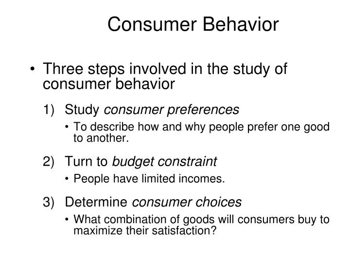
Consumer Behavior. Three steps involved in the study of consumer behavior 1) Study consumer preferences To describe how and why people prefer one good to another. 2) Turn to budget constraint People have limited incomes. 3) Determine consumer choices

E N D
Consumer Behavior • Three steps involved in the study of consumer behavior 1) Study consumer preferences • To describe how and why people prefer one good to another. 2) Turn to budget constraint • People have limited incomes. 3) Determine consumer choices • What combination of goods will consumers buy to maximize their satisfaction?
Consumer Preferences • A bundle of goods or market basket is a collection of one or more commodities. • A market basket may be preferred over another market basket containing a different combination of goods.
Three Basic Assumptions of Consumer Preferences • Preferences are complete. • Give me any two baskets of goods (A and B), I will be able to tell you on of the followings: • I prefer A to B • I prefer B to A • I am indifferent between A and B.
Three Basic Assumptions of Consumer Preferences • Preferences are transitive. • If I prefer A to B and B to C, I must also prefer A to C. • Non-satiation: Consumers always prefer more of any good to less.
The consumer prefers A to all combinations in the blue box, while all those in the pink box are preferred to A. B H E A D G Preferences over Market Basket Clothing (units per week) 50 40 30 20 10 Food (units per week) 10 20 30 40
B H E A D U1 G Indifference Curve Indifference curves represent all combinations of bundles that provide the same level of satisfaction to a person. Clothing (units per week) 50 40 • Combination B,A, & D • yield the same satisfaction • E is preferred to U1 • U1is preferred to H & G 30 20 10 Food (units per week) 10 20 30 40
B H E A D G Indifference Curve Indifference curves slope downward to the right. If it sloped upward it would violate the assumption that more of any commodity is preferred to less. Clothing (units per week) Any market basket lying above and to the right of an indifference curve is preferred to any market basket that lies on the indifference curve. 50 40 30 20 U1 10 Food (units per week) 10 20 30 40
U3 U2 U1 Indifference Map An indifference map is a set of indifference curves that describes a person’s preferences for all combinations of two commodities. Clothing (units per week) Each indifference curve in the map shows the market baskets among which the person is indifferent. D B A Market basket A is preferred to B. Market basket B is preferred to D. Food (units per week)
U1 U2 Indifference Curve Indifference Curves Cannot Cross Clothing (units per week) If crossed, the consumer should be indifferent between A, B and D. However, B contains more of both goods than D. A B D Food (units per week)
A B D E G The Amount of Clothing Given up per Unit of Food Decreases with Food Increase Clothing (units per week) 16 Observation: The amount of clothing given up for a unit of food decreases from 6 to 1. 14 -6 12 10 8 -4 6 -2 4 -1 2 Food (units per week) 1 2 3 4 5
Marginal Rate of Substitution The marginal rate of substitution (MRS) quantifies the amount of one good a consumer will give up to obtain more of another good A Clothing (units per week) 16 14 MRS = 6 -6 12 MRS is measured by the slope of the indifference curve: 10 B 1 8 D MRS = 2 6 E -2 4 1 2 Food (units per week) 1 2 3 4 5
Diminishing Marginal Rate of Substitution Along an indifference curve there is a diminishing marginal rate of substitution. A Clothing (units per week) 16 14 MRS = 6 Indifference curves are convex because as more of one good is consumed, a consumer would prefer to give up fewer units of a second good to get additional units of the first one. -6 12 10 B 1 8 D MRS = 2 6 => Consumers like variety. E -2 4 1 2 Food (units per week) 1 2 3 4 5
Perfect Substitutes Apple juice (glasses) Perfect Substitutes 4 3 Two goods are perfect substitutes when the marginal rate of substitution of one good for the other is constant. 2 1 Orange juice (glasses) 0 1 2 3 4
Perfect Complements Left Shoes Perfect Complements 4 3 Two goods are perfect complements when the indifference curves for the goods are shaped as right angles. 2 1 0 1 2 3 4 Right Shoes
Consumer Choice • Consumers choose a combination of goods that will maximize the satisfaction they can achieve, given the limited budget available to them.
Consumer Choice • The maximizing bundle must satisfy two conditions: 1) It must be located on the budget line. 2) It must give the consumer the most preferred combination of goods and services.
Market basket D cannot be attained given the current budget constraint. D U3 Budget Line Consumer Choice Clothing (units per week) Pc= $2 Pf = $1 I = $80 40 30 20 0 20 40 80 Food (units per week)
Pc= $2 Pf = $1 I = $80 B Budget Line U1 Consumer Choice Clothing (units per week) Point B does not maximize satisfaction because there exist a point A which is attainable and yields a higher satisfaction. Note that the MRS (-(-10/10) = 1 is greater than the price ratio (1/2). 40 30 -10C A 20 +10F 0 20 40 80 Food (units per week)
At market basket A the budget line and the indifference curve are tangent and no higher level of satisfaction can be attained. A At A: MRS =Pf/Pc = .5 U2 Budget Line Consumer Choice Pc= $2 Pf = $1 I = $80 Clothing (units per week) 40 30 20 0 20 40 80 Food (units per week)
Consumer Choice Recall, the slope of an indifference curve is: Further, the slope of the budget line is:
Consumer Choice • Therefore, it can be said that satisfaction is maximized where: • Satisfaction is maximized when the marginal rate of substitution (of F and C) is equal to the ratio of the prices (of F and C). Opportunity cost of food in terms of cloth. Benefit of consuming food as compared to cloth.
INDIFFERENCE CURVES Figure A11.1 shows an indifference curve and map.
INDIFFERENCE CURVES In part (a), Tina is equally happy consuming at any point along the green indifference curve.
INDIFFERENCE CURVES Point C is neither better nor worse than any other point along the indifference curve.
INDIFFERENCE CURVES Points below the indifference curve are worse than points on the indifference curve—are not preferred.
INDIFFERENCE CURVES Points above the indifference curve are better than points on the indifference curve—are preferred.
INDIFFERENCE CURVES Part (b) shows three indifference curves—I0, I1, and I2—that are part of Tina’s indifference map.
INDIFFERENCE CURVES The indifference curve in part (a) is curve I1 in part (b). Tina is indifferent between points C and G.
INDIFFERENCE CURVES Tina prefers point J to points C and G. And she prefers C and G to any point on curve I0.
INDIFFERENCE CURVES • Marginal Rate of Substitution • The marginal rate of substitution is the rate at which a person will give up good y (the good measured on the y-axis) to get more of good x (the good measured on the x-axis) and at the same time remain on the same indifference curve. • Diminishing marginal rate of substitution is the general tendency for the marginal rate of substitution to decrease as the consumer moves down along the indifference curve, increasing consumption of good x and decreasing consumption of good y.
INDIFFERENCE CURVES Figure A11.2 shows the calculation of the marginal rate of substitution. The marginal rate of substitution (MRS) is the magnitude of the slope of an indifference curve. First, we’ll calculate the MRS at point C.
INDIFFERENCE CURVES Draw a straight line with the same slope as the indifference curve at point C. The slope of this line is 8 packs of gum divided by 4 bottles of water, which equals 2 packs of gum per bottle of water.
INDIFFERENCE CURVES This number is Tina’s marginal rate of substitution. Her MRS = 2. At point C, when she consumes 2 bottles of water and 4 packs of gum, Tina is willing to give up gum for water at the rate of 2 packs of gum per bottle of water.
INDIFFERENCE CURVES The red line at point G tells us that Tina is willing to give up 4 packs of gum to get 8 bottles of water. Now calculate Tina’s MRS at point G. Her marginal rate of substitution at point G is 4 divided by 8, which equals 1 ⁄2.
INDIFFERENCE CURVES • Tina’s Equilibrium • The goal of the Tina is to buy the affordable quantities of water and gum that make the her as well off as possible. • Her preference map describe the way a she values different combinations of goods. • Budget and the prices of the water and gum limit her choices.
INDIFFERENCE CURVES Figure A11.3 shows Tina’s equilibrium. Tina’s indifference curves describe her preferences. Tina’s budget line describes the limits to what she can afford. Tina’s best affordable point is C. At that point, she is on her budget line and also on the highest attainable indifference curve.
INDIFFERENCE CURVES Tina can consume the same quantity of water at point J but less gum. She prefers C to J. Point J is equally preferred to points F and H, which Tina can also afford. Points on the budget line between F and H are preferred to F and H. And of all those points, C is the best affordable point for Tina.
INDIFFERENCE CURVES • Deriving the Demand Curve • To derive Tina’s demand curve for bottled water: • Change the price of water • Shift the budget line • Work out the new best affordable point
INDIFFERENCE CURVES Figure A11.4 shows how to derive Tina’s demand curve. When the price of water is $1 a bottle, Tina’s best affordable point is C in part (a) and at point A on her demand curve in part (b). When the price of water is 50 cents a bottle, Tina’s best affordable point is K in part (a) and at point B on her demand curve in part (b).
INDIFFERENCE CURVES Tina’s demand curve in part (b) passes through points A and B.