Download
1 / 74
770 likes | 989 Views
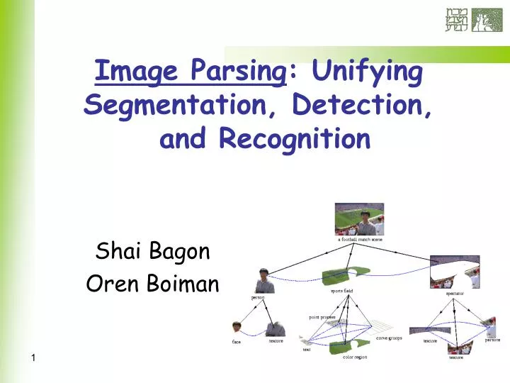
Image Parsing : Unifying Segmentation, Detection, and Recognition. Shai Bagon Oren Boiman. Image Understanding. A long standing goal of Computer Vision Consists of understanding: Objects and visual patterns Context State / Actions of objects Relations between objects Physical layout

E N D
Image Parsing: Unifying Segmentation, Detection, and Recognition Shai Bagon Oren Boiman
Image Understanding • A long standing goal of Computer Vision • Consists of understanding: • Objects and visual patterns • Context • State / Actions of objects • Relations between objects • Physical layout • Etc. A picture is worth a thousand words…
Natural Language Understanding • Very far from being solved • Even NL parsing (syntax) is problematic • Ambiguities requirehigh level (semantic)knowledge
Image Parsing • Decomposition to constituent visual patterns • Edge Detection • Segmentation • Object Recognition
S I Image Parsing Framework High-Level Tasks Object Recognition Classification Generic Framework Low-Level Tasks Segmentation Edge Detection
Top-down(Generative) Constellation, Star-Model etc. Bottom-up(Discriminative) SVM, Boosting, Neural Nets etc. I S Inference: Approach used in “Image Parsing” • + Consistent Solutions • - Slow • + Fast • - Possibly Inconsistent
Coming up next… • Define a (Monstrous) Generative model for Image Parsing • How to perform s-l-o-winference on such models (MCMC) • How to accelerate inference using bottom-up cues (DDMCMC)
Image Parsing Generative Model Uniform S • No. of regions K • Region Shapes Liand Types ζi • Region Parameters Θi Uniform I
Generic Regions Gray level histogram Constant up to Gaussian noise Quadratic form
Faces • Use a PCA model (Eigen-faces) • Estimate Cov. Σ and prin. comp.
Text region shapes • Use Spline templates • Allow Affine transformation • Allow small deformations of control point • Shading intensity model
Problem Formulation • Now we can compute • We’d like to optimize • over the space ofparse graphs
Optimizing P(S|I) is not easy… Rules out gradient methods • Hybrid State Space: Continuous & Discrete • Enormous number of local maxima • Graphical model structure is not pre-determined Rules out Belief propagation
Optimize by Sampling! • Monte Carlo Principle • Use random samples to optimize! • Lets say we’re given N samples from P(S|I) • S1,…,SN • Compute P(Si|I) • Given Si it is easy to compute P(Si|I) • Choose the best Si !
Detour: Sampling methods • How to sample from (very) complex probability space • Sampling algorithm • Why is Markov Chained in Monte Carlo?
Example • Sample from
Markov Chain • A sequence of RandomVariables • Markov property • Transition Given the present The future is independent of the past
Markov Chain – cont. • Under certain conditionsMC converges to unique distribution • Stationary distribution – first eigen-vector of K
Markov Chain Monte Carlo • Reminder: • Had we wanted a sample from Take the value of Xt, • How to make our the stationary distribution of MC ? • How to guarantee convergence ?
Markov Chain convergence • Irreducibility: • The walk can reach any statestarting at any state • Non-periodicity • Stationary distribution cannot depend on t
How to make p(x) Stationary • Detailed Balance: (stationary distribution), if • Written as matrix product • Sufficient condition to converge to p(x) Backward step Independent of x* Probability sum to 1 Forward step The same distribution p(.)
Kernel Selection • Detailed Balance requires Kernel: • Metropolis-Hastings Kernel: • Proposal: where to go next • Acceptance: should we go • MH Kernel provides detailed balance Among the ten most influencing algorithms in science and engineering
Metropolis Hastings • Sample x*~q(x*|xt) • Compute acceptance probability • If rand<A, • Else,
Can we use any q(.) ? 1. Easy to sample from: • we sample from q(.) instead of p(.)
p(x) q(x) Can we use any q(.) ? 2. Supports p(x)
p(x) q(x) Can we use any q(.) ? 3. Explores p(x) wisely: • Too narrow q(.): q(x*|x) ~ N(x, .1) • Too wide q(.): q(x*|x) ~ N(0,20)
Can we use any q(.) ? • Easy to sample from: • we sample from q(.) instead of p(.) • Supports p(x) • Explores p(x) wisely: • q(.) too narrow • q(.) too wide -> low acceptance • The best q(.) is p(.) – but we can’t sample p(.) directly.
Combining Kernels • Suppose we have Satisfying detailed balance with the same • Then also satisfies detailed balance.
Combining MH Kernels • The same applies to Metropolis Hastings Kernels: • Combining MH Kernels with different proposals – MC will converge to
Example Revisited • Proposal distribution: • Acceptance: Given x - easy to compute p(x) Normalization factor cancels out
MAP Estimation • Converge to • Simulated Annealing: • explore less – exploit more! • As the density is peaked at the global maxima
Annealing - example • As the density is peaked at the global maxima
Model Selection • Dimensionality variation in our space • Cannot directly comparedensity of differentstates! Varying number of regions Varying types of explanations per region
Jump across dimensions • Pair-wise common measure
Reversible Jumps • Common measure • Sample extensions u and u* s.tdim(u)+dim(x) = dim(u*)+dim(x*) • Use common dimension for comparison using invertible deterministic functions h and h’ • Explicitly allow reversible jumps x* x
MCMC Summary • Sample p(x) using Markov Chain • Proposal q(x*|x) • Supports p(x) • Guides the sampling • Detailed balance • MH Kernel ensures convergence to p(x) • Reversible Jumps • Comparing across models and dimensions
MCMC – Take home message If you want to make a new sample, You should first learn how to propose. Acceptance is random Eventually you’ll get trapped in endless chains until you become stationary. Some say it is better to do reversible jumps between models.
Back to image parsing • A state is a parse tree • Moves betweenpossible parsesof the image Varying number of regions Different region types: Text, Face and Generic Varying number of parameters
MCMC Moves • Birth / Death of a Face / Text • Split / Merge of a generic region • Model switching for a region • Region boundary evolution
Moves -> Kernel MCMC Moves • Birth / Death of a Face / Text • Split / Merge of a generic region • Model switching for a region • Region boundary evolution
Moves -> Kernel Dimensionality change: must allow reversible jump Text Sub-Kernel Face Sub-Kernel Generic Sub-Kernel Text Birth Text Death Face Birth Face Death Split Region Merge Region Model Switching Boundary Evolution
Using bottom-up cues • So far we haven’t stated the proposal probabilities q(.) • If q(.) is uninformed of the image, convergence can be painfully slow • Solution: use the image to propose moves Face birth kernel
Data Driven MCMC • Define proposal probabilitiesq(x*|x;I) • The proposal probabilities will depend on discriminative tests • Faces detection • Text detection • Edge detection • Parameter clustering • Generative model with Discriminative proposals
Face/Text Detection • Bottom-up cues: AdaBoost • hard classification • Estimate posterior instead • Run on sliding windows at several scales
Edge Map • Canny edge detection at several scales • Only these edges for split / merge
Parameters clustering • Estimate likely parameter settings in the image • Cluster using Mean-Shift
How to propose? • q(S*|S,I) should approximate p(S*|I) • Choose one sub-kernel at random • (e.g., create face) • Use bottom-up cues to generate proposals: S1,S2,… • Weight proposal according to p(Si|I) • Sample from discrete distribution
Generic region – split/merge • Split/merge according to edge map • Dimensionality change – reversible S’ S
Generic region – split/merge • Splitting k into i,j: Sk -> Sij • Proposals are weighted • Normalize weight to probabilities • Sample