Download
1 / 98
1.09k likes | 1.69k Views
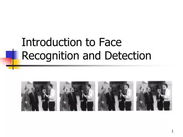
Introduction to Face Recognition and Detection. Outline. Face recognition Face recognition processing Analysis in face subspaces Technical challenges Technical solutions Face detection Appearance-based and learning based approaches Neural networks methods AdaBoost-based methods

E N D
Outline • Face recognition • Face recognition processing • Analysis in face subspaces • Technical challenges • Technical solutions • Face detection • Appearance-based and learning based approaches • Neural networks methods • AdaBoost-based methods • Dealing with head rotations • Performance evaluation
Face Recognition by Humans • Performed routinely and effortlessly by humans • Enormous interest in automatic processing of digital images and videos due to wide availability of powerful and low-cost desktop embedded computing • Applications: • biometric authentication, • surveillance, • human-computer interaction • multimedia management
Face recognition Advantages over other biometric technologies: • Natural • Nonintruisive • Easy to use Among the six biometric attributes considered by Hietmeyer, facial features scored the highest compatibility in a Machine Readable Travel Documents (MRTD) system based on: • Enrollment • Renewal • Machine requirements • Public perception
Classification A face recognition system is expected to identify faces present in images and videos automatically. It can operate in either or both of two modes: • Face verification (or authentication): involves a one-to-one match that compares a query face image against a template face image whose identity is being claimed. • Face identification (or recognition): involves one-to-many matches that compares a query face image against all the template images in the database to determine the identity of the query face. First automatic face recognition system was developed by Kanade 1973.
Outline • Face recognition • Face recognition processing • Analysis in face subspaces • Technical challenges • Technical solutions • Face detection • Appearance-based and learning based approaches • Preprocessing • Neural networks and kernel-based methods • AdaBoost-based methods • Dealing with head rotations • Performance evaluation
Face recognition processing • Face recognition is a visual pattern recognition problem. • A face is a three-dimensional object subject to varying illumination, pose, expression is to be identified based on its two-dimensional image ( or three- dimensional images obtained by laser scan). • A face recognition system generally consists of 4 modules - detection, alignment, feature extraction, and matching. • Localization and normalization (face detection and alignment) are processing steps before face recognition (facial feature extraction and matching) is performed.
Face recognition processing • Face detection segments the face areas from the background. • In the case of video, the detected faces may need to be tracked using a face tracking component. • Face alignment is aimed at achieving more accurate localization and at normalizing faces, whereas face detection provides coarse estimates of the location and scale of each face. • Facial components and facial outline are located; based on the location points, • The input face image is normalized in respect to geometrical properties, such as size and pose, using geometrical transforms or morphing, • The face is further normalized with respect to photometrical properties such as illumination and gray scale.
Face recognition processing After a face is normalized, feature extraction is performed to provide effective information that is useful for distinguishing between faces of different persons and stable with respect to the geometrical and photometrical variations. For face matching, the extracted feature vector of the input face is matched against those of enrolled faces in the database; it outputs the identity of the face when a match is found with sufficient confidence or indicates an unknown face otherwise.
Face recognition processing Face recognition processing flow.
Outline • Face recognition • Face recognition processing • Analysis in face subspaces • Technical challenges • Technical solutions • Face detection • Appearance-based and learning based approaches • Preprocessing • Neural networks and kernel-based methods • AdaBoost-based methods • Dealing with head rotations • Performance evaluation
Analysis in face subspaces Subspace analysis techniques for face recognition are based on the fact that a class of patterns of interest, such as the face, resides in a subspace of the input image space: A small image of 64 × 64 having 4096 pixels can express a large number of pattern classes, such as trees, houses and faces. Among the possible “configurations”, only a few correspond to faces. Therefore, the original image representation is highly redundant, and the dimensionality of this representation could be greatly reduced .
Analysis in face subspaces With the eigenface or PCA approach, a small number (40 or lower) of eigenfaces are derived from a set of training face images by using the PCA. A face image is efficiently represented as a feature vector (i.e. a vector of weights) of low dimensionality. The features in such subspace provide more salient and richer information for recognition than the raw image.
Analysis in face subspaces The manifold (i.e. distribution) of all faces accounts for variation in face appearance whereas the nonface manifold (distribution) accounts for everything else. If we look into facial manifolds in the image space, we find them highly nonlinear and nonconvex. The figure (a) illustrates face versus nonface manifolds and (b) illustrates the manifolds of two individuals in the entire face manifold. Face detection is a task of distinguishing between the face and nonface manifolds in the image (subwindow) space and face recognition between those of individuals in the face mainifold. (a) Face versus nonface manifolds. (b) Face manifolds of different individuals.
Examples • The Eigenfaces, Fisherfaces and Laplacianfaces calculated from the face images in the Yale database.
Outline • Face recognition • Face recognition processing • Analysis in face subspaces • Technical challenges • Technical solutions • Face detection • Appearance-based and learning based approaches • Neural networks methods • AdaBoost-based methods • Dealing with head rotations • Performance evaluation
Technical Challenges The performance of many state-of-the-art face recognition methods deteriorates with changes in lighting, pose and other factors. The key technical challenges are: • Large Variability in Facial Appearance: Whereas shape and reflectance are intrinsic properties of a face object, the appearance (i.e. texture) is subject to several other factors, including the facial pose, illumination, facial expression. Intrasubject variations in pose, illumination, expression, occlusion, accessories (e.g. glasses), color and brightness.
Technical Challenges • Highly Complex Nonlinear Manifolds: The entire face manifold (distribution) is highly nonconvex and so is the face manifold of any individual under various changes. Linear methods such as PCA, independent component analysis (ICA) and linear discriminant analysis (LDA) project the data linearly from a high-dimensional space (e.g. the image space) to a low-dimensional subspace. As such, they are unable to preserve the nonconvex variations of face manifolds necessary to differentiate among individuals. • A linear subspace, do not perform well for classifying between face and nonface manifolds and between manifolds of individuals. This limits the power of the linear methods to achieve highly accurate face detection and recognition.
Technical Challenges • High Dimensionality and Small Sample Size: Another challenge is the ability to generalize as illustrated in figure. A canonical face image of 112 × 92 resides in a 10,304-dimensional feature space. Nevertheless, the number of examples per person (typically fewer than 10) available for learning the manifold is usually much smaller than the dimensionality of the image space; a system trained on so few examples may not generalize well to unseen instances of the face.
Outline • Face recognition • Face recognition processing • Analysis in face subspaces • Technical challenges • Technical solutions: • Statistical (learning-based) • Geometry-based and appearance-based • Non-linear kernel techniques • Taxonomy • Face detection • Appearance-based and learning-based approaches • Non-linear and Neural networks methods • AdaBoost-based methods • Dealing with head rotations • Performance evaluation
Technical Solutions • Feature extraction: construct a “good” feature space in which the face manifolds become simpler i.e. less nonlinear and nonconvex than those in the other spaces. This includes two levels of processing: • Normalize face images geometrically and photometrically, such as using morphing and histogram equalization • Extract features in the normalized images which are stable with respect to such variations, such as based on Gabor wavelets. • Pattern classification: construct classification engines able to solve difficult nonlinear classification and regression problems in the feature space and to generalize better.
Technical Solutions Learning-based approach - statistical learning • Learns from training data to extract good features and construct classification engines. • During the learning, both prior knowledge about face(s) and variations seen in the training data are taken into consideration. • The appearance-based approach such as PCA based methods, has significantly advanced face recognition techniques. • They operate directly on an image-based representation (i.e. an array of pixel intensities) and extracts features in a subspace derived from training images.
Technical Solutions Appearance-based approach utilizing geometric features Detects facial features such as eyes, nose, mouth and chin. • Detects properties of and relations (e.g. areas, distances, angles) between the features are used as descriptors for face recognition. Advantages: • economy and efficiency when achieving data reduction and insensitivity to variations in illumination and viewpoint • facial feature detection and measurement techniques are not reliable enough as they are based on the geometric feature based recognition only • rich information contained in the facial texture or appearance is still utilized in appearance-based approach.
Technical Solutions Nonlinear kernel techniques Linear methods can be extended using nonlinear kernel techniques (kernel PCA) to deal with nonlinearly in face recognition. • A non-linear projection (dimension reduction) from the image space to a feature space is performed; the manifolds in the resulting feature space become simple, yet with subtleties preserved. • A local appearance-based feature space uses appropriate image filters, so the distributions of faces are less affected by various changes. Examples: • Local feature analysis (LFA) • Gabor wavelet-based features such as elastic graph bunch matching (EGBM) • Local binary pattern (LBP)
Taxonomy of face recognition algorithms Taxonomy of face recognition algorithms based on pose-dependency, face representation, and features used in matching.
Outline • Face recognition • Face recognition processing • Analysis in face subspaces • Technical challenges • Technical solutions • Face detection • Appearance-based and learning based approaches • Preprocessing • Neural networks and kernel-based methods • AdaBoost-based methods • Dealing with head rotations • Performance evaluation
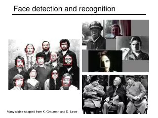
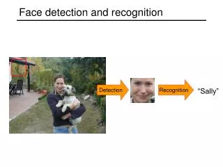
Face detection Face detection is the first step in automated face recognition. Face detection can be performed based on several cues: • skin color • motion • facial/head shape • facial appearance or • a combination of these parameters. Most successful face detection algorithms are appearance-based without using other cues.
Face detection The processing is done as follows: • An input image is scanned at all possible locations and scales by a subwindow. • Face detection is posed as classifying the pattern in the subwindow as either face or nonface. • The face/nonface classifier is learned from face and nonface training examples using statistical learning methods • Note: The ability to deal with nonfrontal faces is important for many real applications because approximately 75% of the faces in home photos are nonfrontal.
Appearance-based and learning based approaches Face detection is treated as a problem of classifying each scanned subwindow as one of two classes (i.e. face and nonface). Appearance-based methods avoid difficulties in modeling 3D structures of faces by considering possible face appearances under various conditions. A face/nonface classifier may be learned from a training set composed of face examples taken under possible conditions as would be seen in the running stage and nonface examples as well. Disadvantage: large variations brought about by changes in facial appearance, lighting and expression make the face manifold or face/non-face boundaries highly complex.
Neural Networks and Kernel Based Methods Nonlinear classification for face detection may be performed using neural networks or kernel-based methods. Neural methods: a classifier may be trained directly using preprocessed and normalized face and nonface training subwindows. • The 24 dimensional feature vector provides a good representation for classifying face and nonface patterns. • In both systems, the neural networks are trained by back-propagation algorithms. Kernel classifiers perform nonlinear classification for face detection using face and nonface examples. • Although such methods are able to learn nonlinear boundaries, a large number of support vectors may be needed to capture a highly nonlinear boundary.
AdaBoost-based Methods The AdaBoost learning procedure is aimed at learning a sequence of best weak classifiers hm(x) and the best combining weights αm. A set of N labeled training examples {(x1, y1), …, (xN, yN)} is assumed available, where yiЄ {+1, -1} is the class label for the example xiЄ Rn.Adistribution [w1, …, wN] of the training examples, where wiis associated with a training example (xi, yi), is computed and updated during the learning to represent the distribution of the training examples. After iteration m, harder-to-classify examples (xi, yi) are given larger weights wi(m), so that at iteration m + 1, more emphasis is placed on these examples. AdaBoost assumes that a procedure is available for learning a weak classifier hm(x) from the training examples, given the distribution [wi(m)].
AdaBoost-based Methods Haar-like features Viola and Jones propose four basic types of scalar features for face detection as shown in figure. Such a block feature is located in a subregion of a subwindow and varies in shape (aspect ratio), size and location inside the subwindow. For a subwindow of size 20 × 20, there can be tens of thousands of such features for varying shapes, sizes and locations. Feature k, taking a scalar value zk(x) Є R, can be considered a transform from the n-dimensional space to the real line. These scalar numbers form an overcomplete feature set for the intrinsically low- dimensional face pattern. Recently, extended sets of such features have been proposed for dealing with out-of-plan head rotation and for in-plane head rotation. These Haar-like features are interesting for two reasons: • powerful face/nonface classifiers can be constructed based on these features • they can be computed efficiently using the summed-area table or integral image technique. Four types of rectangular Haar wavelet-like features. A feature is a scalar calculated by summing up the pixels in the white region and subtracting those in the dark region.
AdaBoost-based Methods Constructing weak classifiers The AdaBoost learning procedure is aimed at learning a sequence of best weak classifiers to combine hm(x) and the combining weights αm. It solves the following three fundamental problems: • Learning effective features from a large feature set • Constructing weak classifiers, each of which is based on one of the selected features • Boosting the weak classifiers to construct a strong classifier
AdaBoost-based Methods Constructing weak classifiers (cont’d) AdaBoost assumes that a “weak learner” procedure is available. The task of the procedure is to select the most significant feature from a set of candidate features, given the current strong classifier learned thus far, and then construct the best weak classifier and combine it into the existing strong classifier. In the case of discrete AdaBoost, the simplest type of weak classifiers is a “stump”. A stump is a single-node decision tree. When the feature is real-valued, a stump may be constructed by thresholding the value of the selected feature at a certain threshold value; when the feature is discrete-valued, it may be obtained according to the discrete label of the feature. A more general decision tree (with more than one node) composed of several stumps leads to a more sophisticated weak classifier.
AdaBoost-based Methods Boosted strong classifier • AdaBoost learns a sequence of weak classifiers hm and boosts them into a strong one HM effectively by minimizing the upper bound on classification error achieved by HM. The bound can be derived as the following exponential loss function: where i is the index for training examples.
AdaBoost learning algorithm AdaBoost learning algorithm
AdaBoost-based Methods FloatBoost Learning AdaBoost attempts to boost the accuracy of an ensemble of weak classifiers. The AdaBoost algorithm solves many of the practical difficulties of earlier boosting algorithms. Each weak classifier is trained stage-wise to minimize the empirical error for a given distribution reweighted according to the classification errors of the previously trained classifiers. It is shown that AdaBoost is a sequential forward search procedure using the greedy selection strategy to minimize a certain margin on the training set. A crucial heuristic assumption used in such a sequential forward search procedure is the monotonicity (i.e. that addition of a new weak classifier to the current set does not decrease the value of the performance criterion). The premise offered by the sequential procedure in AdaBoost breaks down when this assumption is violated. Floating Search is a sequential feature selection procedure with backtracking, aimed to deal with nonmonotonic criterion functions for feature selection. A straight sequential selection method such as sequential forward search or sequential backward search adds or deletes one feature at a time. To make this work well, the monotonicity property has to be satisfied by the performance criterion function. Feature selection with a nonmonotonic criterion may be dealt with using a more sophisticated technique, called plus-L-minus-r, which adds or deletes L features and then backtracks r steps.
FloatBoost algorithm The FloatBoost Learning procedure is composed of several parts: • the training input, • initialization, • forward inclusion, • conditional exclusion and • output. In forward inclusion, the currently most significant weak classifiers are added one at a time, which is the same as in AdaBoost. In conditional exclusion, FloatBoost removes the least significant weak classifier from the set HM of current weak classifiers, subject to the condition that the removal leads to a lower cost than JminM-1. Supposing that the weak classifier removed was the m’-th in HM, then hm’,…,hM-1 and the αm’s must be relearned. These steps are repeated until no more removals can be done. FloatBoost algorithm
AdaBoost-based Methods • Cascade of Strong Classifiers: A boosted strong classifier effectively eliminates a large portion of nonface subwindows while maintaining a high detection rate. Nonetheless, a single strong classifier may not meet the requirement of an extremely low false alarm rate (e.g. 10-6 or even lower). A solution is to arbitrate between several detectors (strong classifier), for example, using the “AND” operation. A cascade of n strong classifiers (SC). The input is a subwindow x. It is sent to the next SC for further classification only if it has passed all the previous SCs as the face (F) pattern; otherwise it exists as nonface (N). x is finally considered to be a face when it passes all the n SCs.
Outline • Face recognition • Face recognition processing • Analysis in face subspaces • Technical challenges • Technical solutions • Face detection • Appearance-based and learning based approaches • Neural networks and kernel-based methods • AdaBoost-based methods • Dealing with head rotations • Performance evaluation
Dealing with Head Rotations Multiview face detection should be able to detect nonfrontal faces. There are three types of head rotation: • out-of-plane rotation (look to the left – to the right) • in-plane rotation (tilted toward shoulders) • up-and-down nodding rotation (up-down) Adopting a coarse-to-fine view-partition strategy, the detector-pyramid architecture consists of several levels from the coarse top level to the fine Bottom level. Rowley et al. propose to use two neural network classifiers for detection of frontal faces subject to in-plane rotation. • The first is the router network, trained to estimate the orientation of an assumed face in the subwindow, though the window may contain a nonface pattern. The inputs to the network are the intensity values in a preprocessed 20 × 20 subwindow. The angle of rotation is represented by an array of 36 output units, in which each unit represents an angular range. • The second neural network is a normal frontal, upright face detector.
Dealing with Head Rotations Coarse-to-fine:The partitions of the out-of-plane rotation for the three-level detector-pyramid is illustrated in figure. Out-of-plane view partition. Out-of-plane head rotation (row 1), the facial view labels (row 2), and the coarse-to-fine view partitions at the three levels of the detector-pyramid (rows 3 to 5).
Dealing with Head Rotations Simple-to-complex: A large number of subwindows result from the scan of the input image. For example, there can be tens to hundreds of thousands of them for an image of size 320 × 240, the actual number depending on how the image is scanned. Merging from different channels. From left to right: Outputs of frontal, left and right view channels and the final result after the merge.
Outline • Face recognition • Face recognition processing • Analysis in face subspaces • Technical challenges • Technical solutions • Face detection • Appearance-based and learning based approaches • Neural networks and kernel-based methods • AdaBoost-based methods • Dealing with head rotations • Performance evaluation
Performance Evaluation The result of face detection from an image is affected by the two basic components: • the face/nonface classifier: consists of face icons of a fixed size (as are used for training). This process aims to evaluate the performance of the face/nonface classifier (preprocessing included), without being affected by merging. • the postprocessing (merger): consists of normal images. In this case, the face detection results are affected by both trained classifier and merging; the overall system performance is evaluated.
Performance Measures • The face detection performance is primarily measured by two rates: the correct detection rate (which is 1 minus the miss detection rate) and the false alarm rate. • As AdaBoost-based methods (with local Haar wavelet features) have so far provided the best face detection solutions in terms of the statistical rates and the speed • There are a number of variants of boosting algorithms: DAB- discrete Adaboost; RAB- real Adaboost; and GAB- gentle Adaboost, with different training sets and weak classifiers. • Three 20-stage cascade classifiers were trained with DAB, RAB and GAB using the Haar-like feature set of Viola and Jones and stumps as the weak classifiers. It is reported that GAB outperformed the other two boosting algorithms; for instance, at an absolute false alarm rate of 10 on the CMU test set, RAB detected only 75.4% and DAB only 79.5% of all frontal faces, and GAB achieved 82.7% at a rescale factor of 1.1.
Performance Measures • Two face detection systems were trained: one with the basic Haar-like feature set of Viola and Jones and one with the extended Haar-like feature set in which rotated versions of the basic Haar features are added. • On average, the false alarm rate was about 10% lower for the extended haar-like feature set at comparable hit rates. • At the same time, the computational complexity was comparable. • This suggests that whereas the larger haar-like feature set makes it more complex in both time and memory in the boosting learning phase, gain is obtained in the detection phase.
Performance Measures Regarding the AdaBoost approach, the following conclusions can be drawn: • An over-complete set of Haar-like features are effective for face detection. The use of the integral image method makes the computation of these features efficient and achieves scale invariance. Extended Haar-like features help detect nonfrontal faces. • Adaboost learning can select best subset from a large feature set and construct a powerful nonlinear classifier. • The cascade structure significantly improves the detection speed and effectively reduces false alarms, with a little sacrifice of the detection rate. • FloatBoost effectively improves boosting learning result. It results in a classifier that needs fewer weaker classifiers than the one obtained using AdaBoost to achieve a similar error rate, or achieve a lower error rate with the same number of weak classifiers. This run time improvement is obtained at the cost of longer training time. • Less aggressive versions of Adaboost, such as GentleBoost and LogitBoost may be preferable to discrete and real Adaboost in dealing with training data containing outliers (distinct, unusual cases). • More complex weak classifiers (such as small trees) can model second-order and/or third-order dependencies, and may be beneficial for the nonlinear task of face detection.
The space of all face images • When viewed as vectors of pixel values, face images are extremely high-dimensional • 100x100 image = 10,000 dimensions • Slow and lots of storage • But very few 10,000-dimensional vectors are valid face images • We want to effectively model the subspace of face images