Download
1 / 23
230 likes | 379 Views
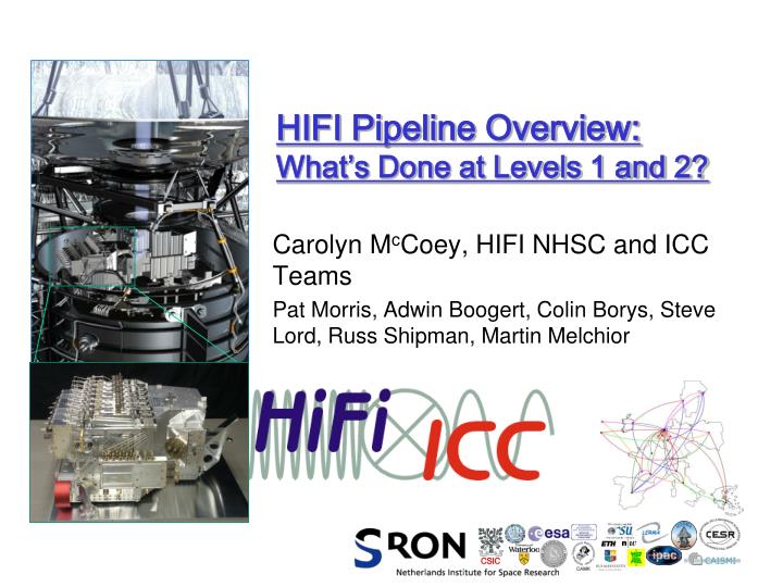
HIFI Pipeline Overview: What’s Done at Levels 1 and 2?. Carolyn M c Coey, HIFI NHSC and ICC Teams Pat Morris, Adwin Boogert, Colin Borys, Steve Lord, Russ Shipman, Martin Melchior. Pipeline Concept.

E N D
HIFI Pipeline Overview: What’s Done at Levels 1 and 2? Carolyn McCoey, HIFI NHSC and ICC Teams Pat Morris, Adwin Boogert, Colin Borys, Steve Lord, Russ Shipman, Martin Melchior
Pipeline Concept • The processing of HIFI observations is similar to ground-based heterodyne telescopes, e.g CSO, JCMT, IRAM, KOSMA… • One pipeline for all HIFI observing modes • The pipeline is customizable
Overall Pipeline Structure Intensity Intensity Intensity
Level 1 Pipeline: Data checks CheckDataStructure, CheckFreqGrid, CheckPhases The initial three steps of the level 1 pipeline are checks that the data have the structure, content and form the patterns that are expected from the observing mode. The CheckFreqGrid step also groups datasets according to LO (local oscillator) tuning and checks for any possible frequency drifts in the data. By default the drift tolerance is set to 5 Hz/s.
Level 1 Pipeline: Bandpass & weights MkFluxHotCold Hot/Cold load measurements are used to obtain the bandpass and receiver temperature. jh and jc are the thermal radiation fields at Th and Tc
The bandpass is used for the intensity calibration, while the receiver temperature can be used for the determination of the channel-dependent weights. If channel weights are not to be determined by the system temperature, then this step of the pipeline can be moved to anywhere before DoFluxHotCold. DoChannelWeights Calculates weights for each channel. The default behaviour is to make use of the receiver temperature from MkFluxHotCold, other possibilities include weighting by integration time, or by the variance of the spectra within a given (moving) window.
Level 1 Pipeline: Reference and Off Subtraction DoRefSubtract Reference measurements taken from blank sky (in DBS modes), from an internal load (in Load Chop modes) or taken at a different LO frequency (in Frequency Switch modes) are subtracted from the source measurements (science datasets) in order to eliminate instrumental drifts from the source measurements. For the Frequency Switch modes, the shifted and the un-shifted spectra are overlaid (with opposite signs) by DoRefSubtract, these spectra need to be folded. Reference measurements are identified by default by the pattern of the observation but you can also choose to use the buffer, chopper or LO values. For more expert users. This step constitutes one half of the double subtraction scheme typical for HIFI.
Level 1 Pipeline: Reference and Off Subtraction • MkOffSmooth • Averages and smoothes (on the frequency scale) the flux data from the OFF measurements. Assumes DoRefSubtract successfully performed. • The default operation of this step is to first take the average over all the spectra included in the OFF dataset and then to smooth the data using a Gaussian filter. • Other options are: • Use a box filter • Apply a polynomial fit after averaging the OFF datasets • Only take the average of the OFF datasets • Average accounting for channel weights or flags, use the frequency scale of the first dataset to be averaged • DoOffSubtract • The calibrated baseline(s) calculated in the MkOffSmooth step are subtracted from the ON measurements of load chop, frequency switch, and position switch modes (on a row-by-row basis for the position switch modes). • In the case of DBS modes, the ON and OFF positions, which both contain science data, are averaged on a scan-by-scan basis. • The interpolation scheme used for the smoothed baseline can be selected: • LINEAR', 'NEAREST', 'PREVIOUS', 'NEXT', 'CUBIC SPLINE'
Level 1 Pipeline: Frequency Calibration DoFluxHotCold The calibrated intensity scale obtained in the MkFluxHotCold task - the bandpass - is applied to the flux data. This transforms the intensity scale to Kelvin units. A choice of interpolation scheme is available. For frequency switch modes, a bandpass is available at both LO frequencies (separated by the LO throw). This makes it possible to consider calibration schemes in which the division of the flux by the bandpass is carried through for each LO frequency separately, i.e. before the DoRefSubtract step. The current calibration scheme applies the DoFluxHotCold after the DoRefSubtract and the bandpass with the same LO frequency as the source phase is used.
‘Scratches’ in some frequency switch and load chop observations seen in WBS-V data. Applying the frequency calibration before the reference position is smoothed and subtracted removes the ‘scratches’ and also improves baseline noise level
Level 1 Pipeline: Velocity Correction DoVelocityCorrection Corrects the frequency scale for the velocity of the spacecraft. A relativistic approach is adopted when correcting for the motion of the spacecraft relative to SSB (Barycentric) or LSR or, in the case of SSOs, relative to the SSO. For non-SSOs, the motion of the sources relative to the LSR or SSB is treated classically. Possible target rest frames to transform to (see parameter targetFrame) are "HSO" (short for Herschel Space Observatory), "GEOCENTRIC", "SSB" or "BARYCENTRIC", "LSR" or "SOURCE”. By default, the task transforms to the "LSR" frame for non SSO's and "SOURCE" for SSO's. An alternative task, which uses a non-relativistic approach and is not a default pipeline step, is DoRadialVelocity
Level 2 Pipeline: Clean up DoCleanUp This step removes all data from the timeline product that are of not of type 'science’ and that correspond to 'ON' measurements. Science datasets that belong to the same LO tuning group and/or the same raster point and/or the same scan line number are merged to form new datasets. You can choose not to merge the datasets.
Level 2 Pipeline: Antenna Temperature DoAntennaTemp This step corrects for all telescope dependent parameters except the coupling of the antenna to the source brightness distribution. TA* = TA’/ηf ηf = 0.96
Level 2 Pipeline: Sideband gains MkSidebandGain This step provides the sideband gains coefficients dependent on detector band, sideband, LOF-scale and IF-scale. If you want to work with only the default coefficients 0.5, you can skip this task and call DoSidebandGain without passing a coefficent. DoSidebandGain Divides the flux (at this stage typically an intensity) by the sideband-specific, detector-band specific, LOF- and and IF-dependent gain coefficients
Level 2 Pipeline: USB/LSB Frequency ConvertFrequencyTask Spectra are transformed from the IF frequency scale to sideband frequencies. For detector bands 1-5 this is defined by: fusb = fLO + fIF and flsb = fLO - fIF For bands 6 and 7, it is: fusb = fLO + CF - fIF and flsb = fLO = CF + fIF where the conversion factor CF is given by 10.4047 GHz for horizontal and 10.4032 GHz for vertical polarization. At the same time, the units are changed from MHz to GHz. This task can also be used to convert data to velocity scale
Level 2 Pipeline: Resample MkFreqGrid This step creates a linear frequency grid that can be used by the DoFreqGrid task to resample the spectra to. By default, the width between successive grid points is set to 0.5 MHz for WBS data, while for HRS data it is determined by inspecting the input spectra. DoFreqGrid Resamples the all HIFI spectra to the frequency grid specified as an input task parameter. By default, the grid determined in the MkFreqGrid step is used. The resampling scheme is set as a trapezoidal integration scheme in combination with a linear interpolation scheme. By default the flux values in the output grid are resampled using an Euler scheme.
Level 2 Pipeline: Cube creation DoGridding The doGridding task is used to create cubes for all mapping mode data. By default, the pipeline assumes a half beam pixel size so if you requested a different beam spacing you will need to re-run the doGridding task with an appropriate beam size. The quality of data cubes may be improved by performing baseline and/or standing wave corrections prior to gridding the data.
Level 2 Pipeline: Averaging DoAverage Computes the average over different scans that belong to the same LO tuning group (frequency surveys), the same raster column and row (in raster maps), or the same line number in OTF maps. Furthermore, science data from ON or OFF are not mixed. Various different options for how to do the average and for pre-selecting the scans to be averaged are available but the default in the standard pipeline is to return a single dataset for each of the conditions described above.
Documentation • “What was done to my data”, in the HIFI User Manual, for a summary of the pipeline steps • HIFI Pipeline Specification document for a detailed description of each pipeline step including the assumptions, mathematics/algorithms and changes to data