Download
1 / 17
170 likes | 358 Views
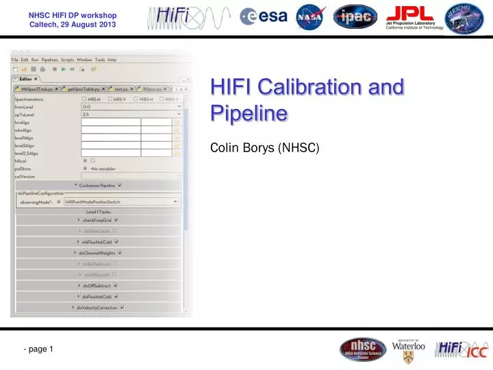
HIFI Calibration and Pipeline. Colin Borys (NHSC). Outline. Why would it be necessary to reprocess data? Take advantage of new calibrations Take advantage of improved pipelines Adjust parameters in existing pipeline Reprocess data after cleaning Basic overview of the pipeline

E N D
HIFI Calibration and Pipeline Colin Borys (NHSC)
Outline • Why would it be necessary to reprocess data? • Take advantage of new calibrations • Take advantage of improved pipelines • Adjust parameters in existing pipeline • Reprocess data after cleaning • Basic overview of the pipeline • What is done at each level • How to reprocess HIFI data (Demos) • HSC on-demand re-processing • Command line based • GUI based re-pipelining (configurable) • Script based re-pipelining
Data by Level Level -1 • Raw data from telescope • Users do not have access to this Level 0 • Data frames and telemetry frames merged • Pointing product applied • Data from proposal system added. Level 0.5 • Spectrometer specific pipelines • Frequency calibration Level 1 • ‘Generic’ pipeline • Flux calibration and reference subtraction Level 2 • Gain and velocity corrections applied • Data averaged • Data split into LSB and USB Level 2.5 • Decon (sscan) • Cubes (mapping)
Some pointers about HIFI frequencies • From channel number to IF frequencies • The assignment of spectrometer channel number to IF frequency is performed in the WBS and HRS branch of the pipeline (between L0 and L0.5) • Space-craft radial velocity • The correction of the space-craft velocity along the source line-of-sight is done in the L1 pipeline • For fixed target, it brings the frequency scale in the LSR • For moving targets, it brings the frequency scale into the target frame • USB/LSB scales • The L2 pipeline creates two products: a USB and an LSB spectrum • The two products are not only mirror spectra of one another wrt the LO frequency – intensity calibration can vary (Sideband ratio) • Velocity scales • No pipeline product is given in velocity scale • Conversion to velocity scale can be done by the user, e.g. in HIPE.
Common use-cases • Data cleaning at level 2 • Flagging of bad channels and/or spectra • Baseline and/or fringe removal • Data cleaning at level 1 • Flagging of bad spectra before averaging • Applying new calibrations • Less common: • New pipelines • Pointing updates • Modifying pipeline steps or parameters
We are here to help • The HIFI pipeline is actually very stable. • Almost all work on data is done with standalone interactive tools, and not the pipeline. • If you find that you need to adjust parameters or modify the standard pipeline steps, you should consult us first.
Example 1: new pipeline • Compare the SPG meta data against the `what’s new’ web http://herschel.esac.esa.int/twiki/bin/view/Public/HipeWhatsNew
Example 2: changes in calibration • Compare calVersion meta data in the observation context against the list on the HIFI calibration web page. • Cal updates usually tied to major releases but not always. http://herschel.esac.esa.int/twiki/bin/view/Public/HifiCalibrationWeb
HSC on-demand reprocessing • Use HSA web page or via HIPE: Window->Show View->Data Access-> HSA
Example 3: tweaking pipelines • The HIFI Pipeline GUI gives a good overview of the pipeline steps and their options. • Alternatively one can edit the pipeline scripts directly.
Example 4: most common • By far the most common reason for pipelining is to reprocess the data after using one of the following three standalone tools: • flagTool • fitBaseline • fitHifiFringe • Normally done on level 2 data, by re-running the level 2.5 pipeline, one gets a much improved final product. • We now go through a few demos illustrating the use of the HIFI pipeline task.
Data used in this demo • 1342190183: Point Mode DBS with emission in a reference position POSITION Reference Position Target Position Reference Position 1 TIME NOD 1 (ON) 2 180”chop throw 3 (1-2) + (4-3) = (ON) – (OFF) 4 NOD 2 (OFF) 180”chop throw Calibrated Spectrum (blue) OFF Spectrum only (pink)
Data used in this demo • 1342181161: DBS Spectral Scan • No emission in the reference beams • Pipeline performs an extra step compared to point mode • Deconvolution (discussed later) combines the spectra at different frequencies into a single spectra.
DEMOS • Basic command line or GUI use • Updating calibration • Re-pipelining after cleaning data • Modifying the pipeline via a GUI
Data calibration: general concept • The ultimate goal of the data calibration is to recover the original source signal from the total signal measured by the detectors • The detection chain function involves (time-dependent) transformations by the optics, electronics, and the environment between the source and the telescope (esp. the atmosphere for ground-based facilities) C = F [Ssou+ Ssky] + Ctel + Cinst Instrument emission Measured detector counts Telescope + inst. response function Sky signal Telescope emission Source signal Instrument Sky C Telescope
HIFI flux calibration (1) 1 Jsou– JOFF = [Csou–COFF] • HIFI works with differential signals, allowing to cancel out to 1st order the telescope and instrument background (so-called Trec) • The instrument response is expressed as a band-pass function, measured on two internal (hot and cold load) black-bodies • As such, the HIFI data are calibrated as brightness temperature[Jν=Bν(T)] Source and reference counts ηsouηlGinst Instrument response Source and reference brightness temperature (K, Double-Side-Band) Source efficiency Forward efficiency Example of an HIFI band-pass function Coupling to the loads Hot and cold load counts Ch–Cc Ginst = (ηh + ηc - 1)[Jh–Jc]
HIFI flux calibration (2) • The HIFI calibration is thus based on a three points (hot, cold, blank sky OFF) measurement scheme • Unlike for the ground-based radio-telescopes, the OFF is not used for atmosphere calibration, but rather for standing wave mitigation • The rate at which those points are visited depends on the drift characteristics applying to each of the 14 detector bands • The standard HIFI products are calibrated on the so-called TA* scale • Calibration onto a single-side-band scale require correction from the side-band ratio (SBR) • Source coupling correction depends on the source extent compared to the beam – many radio-astronomers convert their data into a main beam temperature: [Jsou–JOFF]DSB [Jsou– JOFF]SSB= SBR Gssb Receiver gain response (unpumped mixer) ηl Tmb = TA* ηmb