Download
1 / 39
420 likes | 763 Views
Energy Bands in Solids: Part II. Physics 355. Nomenclature. For most purposes, it is sufficient to know the E n ( k) curves - the dispersion relations - along the major directions of the reciprocal lattice .

E N D
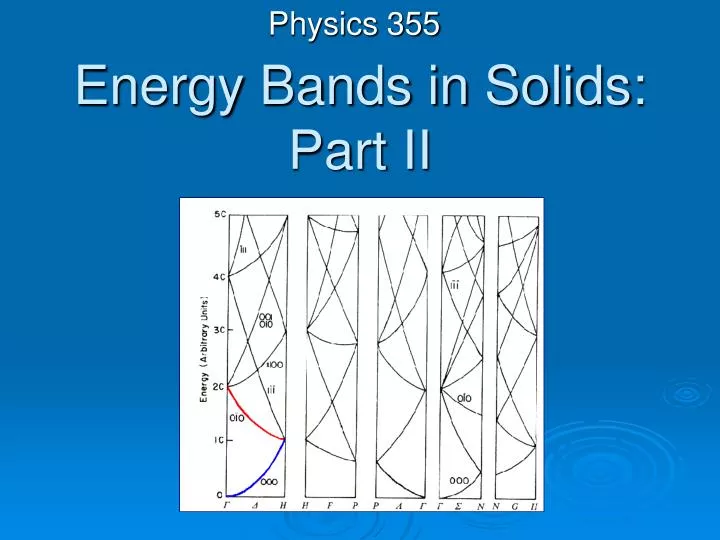
Energy Bands in Solids: Part II Physics 355
Nomenclature For most purposes, it is sufficient to know the En(k) curves - the dispersion relations - along the major directions of the reciprocal lattice. This is exactly what is done when real band diagrams of crystals are shown. Directions are chosen that lead from the center of the Wigner-Seitz unit cell - or the Brillouin zones - to special symmetry points. These points are labeled according to the following rules: • Points (and lines) inside the Brillouin zone are denoted with Greek letters. • Points on the surface of the Brillouin zone with Roman letters. • The center of the Wigner-Seitz cell is always denoted by a G
Nomenclature For cubic reciprocal lattices, the points with a high symmetry on the Wigner-Seitz cell are the intersections of the Wigner Seitz cell with the low-indexed directions in the cubic elementary cell. simple cubic
Nomenclature We use the following nomenclature: (red for fcc, blue for bcc): The intersection point with the [100] direction is calledX(H) The line G—X is called D.The intersection point with the [110] direction is calledK(N) The line G—K is called S.The intersection point with the [111] direction is calledL(P) The line G—L is called L. Brillouin Zone for fcc is bcc and vice versa.
Nomenclature We use the following nomenclature: (red for fcc, blue for bcc): The intersection point with the [100] direction is calledX(H) The line G—X is called D.The intersection point with the [110] direction is calledK(N) The line G—K is called S.The intersection point with the [111] direction is calledL(P) The line G—L is called L.
Electron Energy Bands in 3D Real crystals are three-dimensional and we must consider their band structure in three dimensions, too. Of course, we must consider the reciprocal lattice, and, as always if we look at electronic properties, use the Wigner-Seitz cell (identical to the 1st Brillouin zone) as the unit cell. There is no way to express quantities that change as a function of three coordinates graphically, so we look at a two dimensional crystal first (which do exist in semiconductor and nanoscale physics). The qualitative recipe for obtaining the band structure of a two-dimensional lattice using the slightly adjusted parabolas of the free electron gas model is simple:
LCAO: Linear Combination of Atomic Orbitals • AKA: Tight Binding Approximation • Free atoms brought together and the Coulomb interaction between the atom cores and electrons splits the energy levels and forms bands. • The width of the band is proportional to the strength of the overlap (bonding) between atomic orbitals. • Bands are also formed from p, d, ... states of the free atoms. • Bands can coincide for certain k values within the Brillouin zone. • Approximation is good for inner electrons, but it doesn’t work as well for the conduction electrons themselves. It can approximate the d bands of transition metals and the valence bands of diamond and inert gases.
Electron Energy Bands in 3D The lower part (the "cup") is contained in the 1st Brillouin zone, the upper part (the "top") comes from the second BZ, but it is folded back into the first one. It thus would carry a different band index. This could be continued ad infinitum; but Brillouin zones with energies well above the Fermi energy are of no real interest. These are tracings along major directions. Evidently, they contain most of the relevant information in condensed form. It is clear that this structure has no band gap.
LCAO: Linear Combination of Atomic Orbitals Electronic structure calculations such as our tight-binding method determine the energy eigenvalues n at some point k in the first Brillouin zone. If we know the eigenvalues at all points k, then the band structure energy (the total energy in our tight-binding method) is just where the integral is over the occupied states of below the Fermi level.
Tight Binding Model • The full Hamiltonian of the system is approximated by using the Hamiltonians of isolated atoms, each one centered at a lattice point. • The eigenfunctions are assumed to have amplitudes that go to zero as distances approach the lattice constant. • The assumption is that any necessary corrections to the atomic potential will be small. • The solution to the Schrodinger equation for this type of single electron system, which is time-independent, is assumed to be a linear combination of atomic orbitals.
Band Structure: KCl We first depict the band structure of an ionic crystal, KCl. The bands are very narrow, almost like atomic ones. The band gap is large around 9 eV. For alkali halides they are generally in the range 7-14 eV.
+ + + + + + + + + + + + + + + + + + + + + + + + + Electron Density of States: Free Electron Model Schematic model of metallic crystal, such as Na, Li, K, etc. The equilibrium positions of the atomic cores are positioned on the crystal lattice and surrounded by a sea of conduction electrons. For Na, the conduction electrons are from the 3s valence electrons of the free atoms. The atomic cores contain 10 electrons in the configuration: 1s22s2p6.
Electron Density of States: Free Electron Model • Assume N electrons (1 for each ion) in a cubic solid with sides of length L – particle in a box problem. • These electrons are free to move about without any influence of the ion cores, except when a collision occurs. • These electrons do not interact with one another. • What would the possible energies of these electrons be? 0 L
Electron Density of States: Free Electron Model • How do we know there are free electrons? • You apply an electric field across a metal piece and you can measure a current – a number of electrons passing through a unit area in unit time. • But not all metals have the same current for a given electric potential. Why not?
Electron Density of States The electron density of states is a key parameter in the determination of the physical phenomena of solids. Knowing the energy levels, we can count how many energy levels are contained in an interval DE at the energy E. This is best done in k - space. In phase space, a surface of constant energy is a sphere as schematically shown in the picture. Any "state", i.e. solution of the Schrodinger equation with a specific k, occupies the volume given by one of the little cubes in phase space. The number of cubes fitting inside the sphere at energy E thus is the number of all energy levels up to E.
Electron Density of States: Free Electrons Counting the number of cells (each containing one possible state of ) in an energy interval E, E + DE thus correspond to taking the difference of the numbers of cubes contained in a sphere with "radius" E + DE and of “radius” E. We thus obtain the density of statesD(E) as where N(E) is thenumber of states between E = 0 and E per volume unit; and V is the volume of the crystal.
Electron Density of States: Free Electrons The volume of the sphere in k-space is The volume Vkof one unit cell, containing two electron states is The total number of states is then
From thermodynamics, the chemical potential, and thus the Fermi Energy, is related to the Helmholz Free Energy: where
Electron Density of States: Free Electron Model Chemical Potential If an electron is added, it goes into the next available energy level, which is at the Fermi energy. It has little temperature dependence. m Fermi-Dirac Distribution For lower energies, f goes to 1. For higher energies, f goes to 0.
Free Electron Model: QM Treatment where nx, ny, and nz are integers
Free Electron Model: QM Treatment and similarly for y and z, as well
Free Electron Model: QM Treatment Energy Fermi Energy Velocity
Free Electron Model: QM Treatment million meters per second Fermi Temperature
Free Electron Model: QM Treatment The number of orbitals per unit energy range at the Fermi energy is approximately the total number of conduction electrons divided by the Fermi energy.
Free Electron Model: QM Treatment This represents how many energies are occupied as a function of energy in the 3D k-sphere. As the temperature increases above T = 0 K, electrons from region 1 are excited into region 2.
Electron Density of States: LCAO If we know the band structure at every point in the Brillouin zone, then the DOS is given by the formula where the integral is over the surface Sn() is the surface in k space at which the nth eigenvalue has the value n. Obviously we can not evaluate this integral directly, since we don't know n(k) at all points; and we can only guess at the properties of its gradient. One common approximation is to use the tetrahedron method, which divides the Brillouin zone into (surprise) tetrahedra, and then linearly interpolate within the tetrahedra to determine the gradient. This method is an approximation, but its accuracy obviously improves as we increase the number of k-points.
Electron Density of States: LCAO When the denominator in the integral is zero, peaks due to van Hove singularities occur. Flat bands give rise to a high density of states. It is also higher close to the zone boundaries as illustrated for a two dimensional lattice below. Leon van Hove
Electron Density of States: LCAO • For the case of metals, the bands are very free electron-like (remember we compared with the empty lattice) and the conduction bands are partly filled. • The figure shows the DOS for the cases of a metal , Cu, and a semiconductor Ge. Copper has a free electron-like s-band, upon which d-bands are superimposed. The peaks are due to the d-bands. For Ge the valence and conduction bands are clearly seen.
Electron Density of States: LCAO fcc The basic shape of the density of states versus energy is determined by an overlap of orbitals. In this case s and d orbitals…
Electron Density of States: LCAO bcc tungsten