Chapter 5 Discrete Probability Distribution

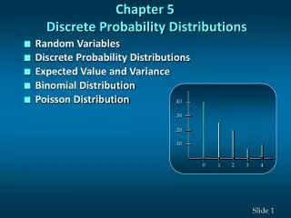
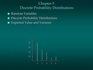
1. I. Basic Definitions • II. Summary Measures for Discrete Random Variable • Expected Value (Mean) • Variance and Standard Deviation • III. Two Popular Discrete Probability Distributions • Binomial Distribution • Poisson Distribution Chapter 5 Discrete Probability Distribution

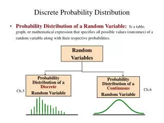
2. I. Basic Definitions • Random Variable: (p.195) • a numerical description of the outcomes of an experiment. • Assign values to outcomes of an experiment so the experiment can be represented as a random variable. • Example: • Test scores: 0  X  100 • Toss coin: X = {0, 1} • Roll a die: X = {1, 2, 3, 4, 5, 6}

3. I. Basic Definitions • Discrete Random Variable: It takes a set of discrete values. Between two possible values some values are impossible. • Continuous Random Variable: Between any two possible values for this variable, another value always exists. • Example: • Roll a die: X = {1, 2, 3, 4, 5, 6}. X is a discrete random variable. • Weight of a person selected at random: X is a continuous random variable.

4. I. Basic Definitions • Two ways to present a discrete random variable • Probability Distribution: (p.198 Table 5.3) • a list of all possible values (x) for a random variable and probabilities (f(x)) associated with individual values. • Probability Function: probability may be represented as a function of values of the random variable. • Example: p.199 • Consider the experiment of rolling a die and define the random variable X to be the number coming up. • 1. Probability distribution • 2. Probability function: f(x) = 1/6.

5. I. Basic Definition • Valid Discrete Probability Function • 0  f(x)  1 for all f(x) AND •  f(x) = 1 • Example: p.200 #7 • a. The probability distribution is proper because all f(x) meet requirements 0  f(x)  1 and  f(x) = 1. • b. P(X=30) = f(30) = .25 • c. P(X25) = f(25) + f(20) = .15 + .20 = .35 • d. P(X>30) = f(35) = .40 • Homework: p.201 #10, p.201 #14

6. I. Basic Definitions Example: p.202 #14 a. Find valid f(200): .1+.2+.3+.25+.1+f(200) = 1, so f(200) = .05 b. P(?) P(X>0) = f(50)+f(100)+f(150)+f(200) = .7 c. P(?) P(X100) = f(100)+f(150)+f(200) = .4 (“at least”)

7. II. Summary Measures for Discrete Random Variable • Expected Value (mean): E(X) or  (p.203) • E(X) = xf(x) • Variance: Var(X) or 2 (p.203) • Var(X) = (x-  )2f(x) • Homework: p.204 #16 • Example: Consider the experiment of tossing coin and define X to be 0 if head and 1 if tail. Find the expected value and variance. E(X) = xf(x) = (0)(.5)+(1)(.5) = .5 Var(X) = (x-  )2f(x) = (0 - .5)2(.5)+(1 - .5)2(.5) = .25

8. III. Two Popular Discrete Probability Distributions — Binomial and Poisson Outlines: 1. Probability Distribution: Binomial Distribution: Table 5 (p.989 - p.997). Given n, p, x  f(x). Poisson Distribution: Table 7 (p.999 - p.1004). Given , x  f(x). 2. Applications: Difference between Binomial and Poisson. 3. Applications: criterion to define “success”.

9. III. Two Popular Discrete Probability Distributions • 1. Binomial Distribution p.207 • Random variable X: x “successes” out of n trials (the number of “successes” in n trials). • Three conditions for Binomial distribution: • n independent trials • Two outcomes for each trial: “success” and “failure”. • p: probability of a “success” is a constant from trial to trial.

10. III. Two Popular Discrete Probability Distributions Example: Toss a coin 10 times. We define the “success” as a head and X is the number of heads from 10 trials. Does X have a binomial distribution? Answer: Yes. Follow-up: Why? n? p? Example: Roll a die 10 times. We define the “success” as 5 or more points coming up and X is the number of successes from 10 trials. Does X have a binomial distribution? Answer: Yes. Why? n? p?

11. III. Two Popular Discrete Probability Distributions • Summary Measures for Binomial Distribution • E(X) = np p.214 • Var(X) = np(1-p) p.214 • Binomial Probability Distribution p.212 • — f(x) = P(X=x) = • — Table 5 (p.989-p.997): Given n, p and x, find f(x). • Homework: p.216 #26, #27, #29, #30 c, d.

12. Example: p.216 #25 Given: Binomial, n = 2, p = .4 “Success” X: # of successes in 2 trials Answer: b. f(1) = ? (Table 5) f(1) = .48 c. f(0) = ? f(0) = .36 d. f(2) = ? e. P(X1) = ? f(2) = .16) P(X1) = f(1) + f(2) = .64 e. E(X) = np = .8 Var(X) = np(1-p) = .48  = ?

13. Example: p.217 #35 (Application) Binomial distribution? 1. Is there a criterion for “success” and “failure”? 2. n trials? n=? 3. p=? Given: “Success”: withdraw; n = 20; p = .20 Answer: a. P(X  2) = f(0) + f(1) + f(2) = .0115 + .0576 + .1369 = .2060 b. P(X=4) = f(4) = .2182 c. P(X>3) = 1 - P(X  3) = 1 – [f(0) + f(1) + f(2) + f(3)] = 1 - .0115 - .0576 - .1369 - .2054 = .5886 d. E(X) = np = (20)(.2) = 4.

14. III. Two Popular Discrete Probability Distributions • 2. Poisson Distribution p.218 • Random variable X: x “occurrences” per unit (the number of “occurrences” in a unit - time, size, ...). • Example: X = the number of calls per hour. Does X have a Poisson distribution? • Answer: Yes. Because • “Occurrence”: a call. • Unit: an hour. • X: the number of “occurrences” (calls) per unit (hour). • Reading: p.216 #29, #30, and p.220 #40, p.221 #42 • Binomial or Poisson? If Binomial, “success”? p? n? • If Poisson, “occurrence”? ? unit?

15. III. Two Popular Discrete Probability Distributions • Summary Measures for Poisson Distribution • E(X) =  ( is given) • Var(X) =  • Poisson Probability Distribution p.219 • — f(x) = P(X=x) = • — Table 7 (p.999 through p.1004): Given  and x, find f(x). • Note: Keep the unit of  consistent with the question. • Homework: p.220 #38, p.221 #42, #43

16. Example: p.220 #39 • Given: • Poisson distribution, because • X = the number of occurrences per time period. •  = 2 and unit is “a time period”. • Note: Unit in questions may be different. • Answer: • a. f(x) = = • b. What is the average number of occurrences in • three time periods? (Different unit!) • 3 = (3)( ) = 6. c. f(x) = • d. f(2) = P(X=2) = .2707 (Table 7.  =2, x = 2) • e. f(6) = P(X=6) = .1606 (Table 7.  =6, x = 6)

17. Example: p.221 #43 Given: • Poisson distribution, because • X = the number of arrivals per time period. •  = 10 and unit is “per minute”. • Note: Unit in questions may be different. • Answer: • a. f(0) = 0 (Table 7.  =10, x = 0) • b. P(X3) = f(0)+f(1)+f(2)+f(3) (Table 7.  =10, x = ?) • = 0 + .0005 + .0023 + .0076 = .0104 • c. P(X=0) = f(0) = .0821 • (Table 7.  =(10)(15/60)=2.5 for unit of 15 seconds, x = 0) • d. P(X1) = ? (Table 7.  =2.5, x = ?) • P(X1) = f(1) + f(2) + f(3) + … ??? • = 1 - P(X<1) = 1 - f(0) = 1 - .0821 = .9179.

18. Chapter 5 Summary • Binomial distribution: X = # of “successes” out of n trials • Poisson distribution: X = # of “occurrences” per unit • For Binomial distribution, E(X)=np, Var(X)=np(1-p) • For Poisson distribution, E(X) =  = Var(X) • Binomial distribution table: Table 5 • Poisson distribution table: Table 7 • Poisson Approximation of Binomial distribution • If p  .05 AND n  20, Poisson distribution (Table 7) can • be used to find probability for Binomial distribution. • Example: A Binomial distribution with n = 250 and p = .01, • f(3) = ? • Answer:  = np =(250)(.01)=2.5. From Table 7, f(x)=.2138 • Sampling with replacement and without replacement.

19. Example: A bag of 100 marbles contains 10% red ones. Assume that samples are drawn randomly with replacement. a. If a sample of two is drawn, what is the probability that both will be red? b. If a sample of three is drawn, what is the probability that at least one will be red? (“without replacement”: Hypergeometric distribution p.214) Answer: a. n = 2, p = .1, f(2) = ? From Table 5, f(2) = .01 b. n = 3, p = .1, P(X1) = f(1) + f(2) + f(3) From Table 5, P(X1) = .2430 + .0270 + .0010 = .271