Download
1 / 44
780 likes | 1.68k Views
Chapter 5 Joint Probability Distribution. Introduction. If X and Y are two random variables, the probability distribution that defines their simultaneous behavior is a Joint Probability Distribution. Examples: Signal transmission: X is high quality signals and Y low quality signals.

E N D
Introduction • If X and Y are two random variables, the probability distribution that defines their simultaneous behavior is a Joint Probability Distribution. Examples: • Signal transmission: X is high quality signals and Y low quality signals. • Molding: X is the length of one dimension of molded part, Y is the length of another dimension. • THUS, we may be interested in expressing probabilities expressed in terms of X and Y, e.g., P(2.95 < X < 3.05 and 7.60 < Y < 7.8)
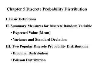
Two discrete random variables • Range of random variables (X,Y) is the set of points (x,y) in 2D space for which the probability that X = x and Y = y is positive. • If X and Y are discrete random variables, the joint probability distribution of X and Y is a description of the set of points (x,y) in the range of (X,Y) along with the probability of each point. • Sometimes referred to as Bivariate probabilitydistribution, or Bivariate distribution.
Figure 5-1Joint probability distribution of X and Y in Example 5-1.
Joint probability mass function • The joint probability mass function of the discrete random variables X and Y, denoted as fXY(x,y) satisfies:
Marginal probability distributions • Individual probability distribution of a random variable is referred to as its Marginal Probability Distribution. • Marginal probability distribution of X can be determined from the joint probability distribution of X and other random variables. • Marginal probability distribution of X is found by summing the probabilities in each column, for Y, summation is done in each row.
Marginal probability distributions (Cont.) • If X and Y are discrete random variables with joint probability mass function fXY(x,y), then the marginal probability mass function of X and Y are where Rxdenotes the set of all points in the range of (X, Y) for which X =x and Rydenotes the set of all points in the range of (X, Y) for which Y =y
Mean and Variance • If the marginal probability distribution of X has the probability function f(x), then • R = Set of all points in the range of (X,Y).
Conditional probability • Given discrete random variables X and Y with joint probability mass function fXY(X,Y), the conditional probability mass function of Y given X = x is fY|x(y) = fXY(x,y)/fX(x) for fX(x) > 0
Conditional probability (Cont.) • Because a conditional probability mass function fY|x(y) is a probability mass function for all y in Rx, the following properties are satisfied: (1) fY|x(y) 0 (2) fY|x(y) = 1 (3) P(Y=y|X=x) = fY|x(y)
Example 5-6: Conditional probability distribution for Y given X
Conditional probability (Cont.) • Let Rx denote the set of all points in the range of (X,Y) for which X=x. The conditional mean of Y given X = x, denoted as E(Y|x) or Y|x, is • And the conditional variance of Y given X = x, denoted as V(Y|x) or 2Y|x is
Independence • For discrete random variables X and Y, if any one of the following properties is true, the others are also true, and X and Y are independent. (1) fXY(x,y) = fX(x) fY(y) for all x and y (2) fY|x(y) = fY(y) for all x and y with fX(x) > 0 (3) fX|y(x) = fX(x) for all x and y with fY(y) > 0 (4) P(X A, Y B) = P(X A)P(Y B) for anysets A and B in the range of X and Y respectively. • If we find one pair of x and y in which the equality fails, X and Y are not independent.
Joint and Marginal probability Conditional probability distribution for X and Y Distribution for X and Y
Rectangular Range for (X, Y) • If the set of points in two-dimensional space that receive positive probability under fXY(x, y) does not form a rectangle, X and Y are not independent because knowledge of X can restrict the range of values of Y that receive positive probability. • If the set of points in two dimensional space that receives positive probability under fXY(x, y) forms a rectangle, independence is possible but not demonstrated. One of the conditions must still be verified.
Two continuous random variables • Analogous to the probability density function of a single continuous random variable, a Joint probability density function can be defined over two-dimensional space.
Joint probability distribution • A joint probability density function for the continuous random variables X and Y, denoted as fXY(x,y), satisfies the following properties: (1) fXY(x,y) 0 for all x, y (2) (3) For any range R of two-dimensional space
Joint probability distribution (Cont.) • The probability that (X,Y) assumes a value in the region R equals the volume of the shaded region.
Joint probability density function for the lengths of different dimensions of an injection-molded part; P(2.95 < X < 3.05,7.60 < Y < 7.80)
Marginal probability distribution • If the joint probability density function of continuous random variables X and Y is fXY(x,y), the marginal probability density function of X and Y are and where Rx denotes the set of all points in the range of (X,Y) for which X = x and Ry denotes the set of all points in the range of (X,Y) for which Y = y.
Marginal probability distribution (Cont.) • A probability involving only one random variable, e.g., P(a < X < b), can be found from the marginal probability of X or from the joint probability distribution of X and Y. • For example: P(a < x < b) = P(a < x < b, - < Y < )=
Mean and variance • E(x) = x = Where Rx denotes the set of all points in the range of (X,Y) for which X=x and Ry denotes the set of all points in the range of (X,Y)
Conditional Probability Distributions • Definition
Covariance and Correlation Expected Value of a Function of TwoRandom Variables:
Example 5-24 Figure 5-12Joint distribution of X and Y for Example 5-24.
Covariance Figure 5-13Joint probability distributions and the sign of covariance between X and Y.
Example 5-26 Figure 5-14Joint distribution for Example 5-26.
Correlation Example 5-28 Figure 5-16Random variables with zero covariance from Example 5-28.
Linear Combinations of Random Variables Mean of a Linear Combination