Download
1 / 39
400 likes | 547 Views
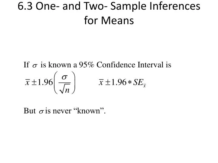
6.3 One- and Two- Sample Inferences for Means. If σ is unknown. Estimate σ by sample standard deviation s The estimated standard error of the mean will be Using the estimated standard error we have a confidence interval of

E N D
If σis unknown • Estimate σby sample standard deviation s • The estimated standard error of the mean will be • Using the estimated standard error we have a confidence interval of • The multiplier needs to be bigger than Z (e.g., 1.96 for 95% CI). The confidence interval needs to be wider to take into account the added uncertainty in using s to estimate s. • The correct multipliers were figured out by a Guinness Brewery worker.
What is the correct multiplier? “t” • 100(1-a)% confidence interval when s is unknown • 95% CI =100(1-0.05)% confidence interval when s is unknown
Properties of t distribution • The value of t depends on how much information we have about s. The amount of information we have about s depends on the sample size. • The information is “degrees of freedom” and for a sample from one normal population this will be: df=n-1.
t curve and z curve Both the standard normal curve N(0,1) (the z distribution), and all t(v)distributions are density curves, symmetric about a mean of 0, but t distributions have more probability in the tails. As the sample size increases, this decreases and the t distribution more closely approximates the z distribution. By n = 1000 they are virtually indistinguishable from one another.
Quantiles of t distribution t table is given in the book: Table B.4 It depends on the degrees of freedom as well df probability t 5 0.90 1.476 10 0.95 1.812 20 0.99 2.528 25 0.975 2.060 ∞ 0.975 1.96
Example • Noise level, n=12 74.0 78.6 76.8 75.5 73.8 75.6 77.3 75.8 73.9 70.2 81.0 73.9 • Point estimate for the average noise level of vacuum cleaners; • 95% Confidence interval
Solution • n=12, • Critical value with df=11 • 95% CI:
On the other hand • t0.95,9 =1.833, t0.05,9 =-1.83 • If we have a test statistic value that is either too small (<-1.83) or too big (>1.83), then we have strong evidence against H0. • t=1.74 which is not too small or too big (compared to the cutoff values above/ ”critical values”) , then we cannot reject the null.
Rejection Region method and p-value method • For Ha: m<m0, if z test statistic is less than -1.645, then the p-value is less than 0.05. Comparing the p-value to 0.05 is the same as comparing the z value to -1.645. • For t tests we can also find some critical values corresponding to level of a that we can compare to our test statistic. • Test statistic in the rejection region is the same as p-value is less than a.
Paired Data 1982 study of trace metals in South Indian River. 6 random locations 5 3 1 6 2 4 T=top water zinc concentration (mg/L) B=bottom water zinc (mg/L) 1 2 3 4 5 6 Top 0.415 0.238 0.390 0.410 0.605 0.609 Bottom 0.430 0.266 0.567 0.531 0.707 0.716
Assumptions: The population of differences follows a normal distribution. A normal plot of differences, d’s, should be fairly straight. Note: We don’t need B or T to be normal.
Rejection region exercise • Tell when to reject H0: μ = 120 using a t-test. Answers would be of the form • reject H0 when t < -1.746 or maybe • reject H0 when |t| > 1.746 or maybe • reject H0 when t > 1.746 • (a) HA: μ < 120, α = 0.05, n=20 • (b) HA: μ > 120, α = 0.10, n=18 • (c) HA: μ ≠ 120, α = 0.01, n=9
Find p-value exercise • Answers would be of the form • 0.10 < p < 0.05 • p < 0.001 • p > 0.8 • After finding the p-value in each case, tell whether • to reject or not reject H0 at the α = 0.05 level. • (a) HA: μ > 120, n=7, t = -2.58 • (b) HA: μ < 120, n=7, t = -2.58 • (c) HA: μ ≠ 120, n=7, t = -2.58