Download
1 / 52
520 likes | 675 Views
Particle Physics Instrumentation. Werner Riegler, CERN, werner.riegler@cern.ch The 2011 CERN – Latin-American School of High-Energy Physics Natal, Brazil, 23 March - 5 April 2011. Lecture3/3 Signals, Electronics, Trigger, DAQ. Cloud Chambers 1910-1950ies. Wilson Cloud Chamber 1911.

E N D
Particle Physics Instrumentation Werner Riegler, CERN, werner.riegler@cern.ch The 2011 CERN – Latin-American School of High-Energy PhysicsNatal, Brazil, 23 March - 5 April 2011 Lecture3/3 Signals, Electronics, Trigger, DAQ W. Riegler/CERN
Cloud Chambers 1910-1950ies Wilson Cloud Chamber 1911 W. Riegler/CERN
Cloud Chamber X-rays, Wilson 1912 Alphas, Philipp 1926 W. Riegler/CERN
Cloud Chamber Magnetic field 15000 Gauss, chamber diameter 15cm. A 63 MeV positron passes through a 6mm lead plate, leaving the plate with energy 23MeV. The ionization of the particle, and its behaviour in passing through the foil are the same as those of an electron. Positron discovery, Carl Andersen 1933 W. Riegler/CERN
Cloud Chamber Particle momenta are measured by the bending in the magnetic field. ‘ … The V0 particle originates in a nuclear Interaction outside the chamber and decays after traversing about one third of the chamber. The momenta of the secondary particles are 1.6+-0.3 BeV/c and the angle between them is 12 degrees … ‘ By looking at the specific ionization one can try to identify the particles and by assuming a two body decay on can find the mass of the V0. ‘… if the negative particle is a negative proton, the mass of the V0 particle is 2200 m, if it is a Pi or Mu Meson the V0 particle mass becomes about 1000m …’ Rochester and Wilson W. Riegler/CERN
Nuclear Emulsion 1930ies to Present Film played an important role in the discovery of radioactivity but was first seen as a means of studying radioactivity rather than photographing individual particles. Between 1923 and 1938 Marietta Blau pioneered the nuclear emulsion technique. E.g. Emulsions were exposed to cosmic rays at high altitude for a long time (months) and then analyzed under the microscope. In 1937, nuclear disintegrations from cosmic rays were observed in emulsions. The high density of film compared to the cloud chamber ‘gas’ made it easier to see energy loss and disintegrations. W. Riegler/CERN
Nuclear Emulsion Discovery of the Pion: The muon was discovered in the 1930ies and was first believed to be Yukawa’s meson that mediates the strong force. The long range of the muon was however causing contradictions with this hypothesis. In 1947, Powell et. al. discovered the Pion in Nuclear emulsions exposed to cosmic rays, and they showed that it decays to a muon and an unseen partner. The constant range of the decay muon indicated a two body decay of the pion. Discovery of muon and pion W. Riegler/CERN
Nuclear Emulsion First evidence of the decay of the Kaon into 3 Pions was found in 1949. Pion Kaon Pion Pion W. Riegler/CERN
Bubble Chamber 1950ies to early 1980ies In the early 1950ies Donald Glaser tried to build on the cloud chamber analogy: Instead of supersaturating a gas with a vapor one would superheat a liquid. A particle depositing energy along it’s path would then make the liquid boil and form bubbles along the track. In 1952 Glaser photographed first Bubble chamber tracks. Luis Alvarez was one of the main proponents of the bubble chamber. The size of the chambers grew quickly 1954: 2.5’’(6.4cm) 1954: 4’’ (10cm) 1956: 10’’ (25cm) 1959: 72’’ (183cm) 1963: 80’’ (203cm) 1973: 370cm W. Riegler/CERN
Bubble Chamber ‘old bubbles’ ‘new bubbles’ Unlike the Cloud Chamber, the Bubble Chamber could not be triggered, i.e. the bubble chamber had to be already in the superheated state when the particle was entering. It was therefore not useful for Cosmic Ray Physics, but as in the 50ies particle physics moved to accelerators it was possible to synchronize the chamber compression with the arrival of the beam. For data analysis one had to look through millions of pictures. W. Riegler/CERN
Bubble Chamber In the bubble chamber, with a density about 1000 times larger that the cloud chamber, the liquid acts as the target and the detecting medium. Figure: A propane chamber with a magnet discovered the S° in 1956. A 1300 MeV negative pion hits a proton to produce a neutral kaon and a S°, which decays into a L° and a photon. The latter converts into an electron-positron pair. W. Riegler/CERN
Bubble Chamber Discovery of the - in 1964 BNL, First Pictures 1963, 0.03s cycle W. Riegler/CERN
Bubble Chamber Gargamelle, a very large heavy-liquid (freon) chamber constructed at EcolePolytechnique in Paris, came to CERN in 1970. It was 2 m in diameter, 4 m long and filled with Freon at 20 atm. With a conventional magnet producing a field of almost 2 T, Gargamelle in 1973 was the tool that permitted the discovery of neutral currents. Can be seen outside the Microcosm Exhibition W. Riegler/CERN
Bubble Chamber The photograph of the event in the Brookhaven 7-foot bubble chamber which led to the discovery of the charmed baryon (a three-quark particle) is shown at left. A neutrino enters the picture from below (dashed line) and collides with a proton in the chamber's liquid. The collision produces five charged particles: A negative muon, three positive pions, and a negative pion and a neutral lambda. The lambda produces a characteristic 'V' when it decays into a proton and a pi-minus. The momenta and angles of the tracks together imply that the lambda and the four pions produced with it have come from the decay of a charmed sigma particle, with a mass of about 2.4 GeV. The detector began routine operations in 1974. The following year, the 7-foot chamber was used to discover the charmed baryon, a particle composed of three quarks, one of which was the "charmed" quark. W. Riegler/CERN
Bubble Chamber 3.7 meter hydrogen bubble chamber at CERN, equipped with the largest superconducting magnet in the world. During its working life from 1973 to 1984, the "Big European Bubble Chamber" (BEBC) took over 6 million photographs. Can be seen outside the Microcosm Exhibition W. Riegler/CERN
Bubble Chambers The excellent position (5m) resolution and the fact that target and detecting volume are the same (H chambers) makes the Bubble chamber almost unbeatable for reconstruction of complex decay modes. The drawback of the bubble chamber is the low rate capability (a few tens/ second). E.g. LHC 109 collisions/s. The fact that it cannot be triggered selectively means that every interaction must be photographed. Analyzing the millions of images by ‘operators’ was a quite laborious task. That’s why electronics detectors took over in the 70ties. W. Riegler/CERN
Detector + Electronics 1925 ‘Über das Wesen des Compton Effekts’ W. Bothe, H. Geiger, April 1925 Bohr, Kramers, Slater Theorie: Energy is only conserved statistically testing Compton effect ‘ Spitzenzähler ’ W. Riegler/CERN
Detector + Electronics 1925 ‘Über das Wesen des Compton Effekts’, W. Bothe, H. Geiger, April 1925 • ‘’Electronics’’: • Cylinders ‘P’ are on HV. • The needles of the counters are insulated and connected to electrometers. • Coincidence Photographs: • A light source is projecting both electrometers on a moving film role. • Discharges in the counters move the electrometers , which are recorded on the film. • The coincidences are observed by looking through many meters of film. W. Riegler/CERN
Detector + Electronics 1929 In 1928 Walther Müller started to study the sponteneous discharges systematically and found that they were actually caused by cosmic rays discovered by Victor Hess in 1911. By realizing that the wild discharges were not a problem of the counter, but were caused by cosmic rays, the Geiger-Müller counter went, without altering a single screw from a device with ‘fundametal limits’ to the most sensitive intrument for cosmic rays physics. ‘ZurVereinfachung von Koinzidenzzählungen’ W. Bothe, November 1929 Coincidence circuit for 2 tubes W. Riegler/CERN
1930 - 1934 Cosmic ray telescope 1934 Rossi 1930: Coincidence circuit for n tubes W. Riegler/CERN
Geiger Counters By performing coincidences of Geiger Müller tubes e.g. the angular distribution of cosmic ray particles could be measured. W. Riegler/CERN
Scintillators, Cerenkov light, Photomultipliers In the late 1940ies, scintillation counters and Cerenkov counters exploded into use. Scintillation of materials on passage of particles was long known. By mid 1930 the bluish glow that accompanied the passage of radioactive particles through liquids was analyzed and largely explained (Cerenkov Radiation). Mainly the electronics revolution begun during the war initiated this development. High-gain photomultiplier tubes, amplifiers, scalers, pulse-height analyzers. W. Riegler/CERN
Antiproton One was looking for a negative particle with the mass of the proton. With a bending magnet, a certain particle momentum was selected (p=mv). Since Cerenkov radiation is only emitted if v>c/n, two Cerenkov counters (C1, C2) were set up to measure a velocity comparable with the proton mass. In addition the time of flight between S1 and S2 was required to be between 40 and 51ns, selecting the same mass. W. Riegler/CERN
Anti Neutrino Discovery 1959 Reines and Cowan experiment principle consisted in using a target made of around 400 liters of a mixture of water and cadmium chloride. The anti-neutrino coming from the nuclear reactor interacts with a proton of the target matter, giving a positron and a neutron. The positron annihilates with an electron of the surrounding material, giving two simultaneous photons and the neutron slows down until it is eventually captured by a cadmium nucleus, implying the emission of photons some 15 microseconds after those of the positron annihilation. + p n + e+ W. Riegler/CERN
Spark Counters The Spark Chamber was developed in the early 60ies. Schwartz, Steinberger and Lederman used it in discovery of the muon neutrino A charged particle traverses the detector and leaves an ionization trail. The scintillators trigger an HV pulse between the metal plates and sparks form in the place where the ionization took place. W. Riegler/CERN
The Electronic Image During the 1970ies, the Image and Logic devices merged into ‘Electronics Imaging Devices’ W. Riegler/CERN
W, Z-Discovery 1983/84 UA1 used a very large wire chamber. Can now be seen in the CERN Microcosm Exhibition This computer reconstruction shows the tracks of charged particles from the proton-antiproton collision. The two white tracks reveal the Z's decay. They are the tracks of a high-energy electron and positron. W. Riegler/CERN
Moore’s Law Moore's law describes a long-term trend in the history of computing hardware. The number of transistors that can be placed inexpensively on an integrated circuit doubles approximately every two years. This trend has continued for more than half a century and is expected to continue until 2015 or 2020 or later. The capabilities of many digital electronic devices are strongly linked to Moore's law: processing speed, memory capacity, sensors and even the number and size of pixels in digital cameras All of these are improving at (roughly) exponential rates as well. This exponential improvement has dramatically enhanced the impact of digital electronics in nearly every segment of the world economy and clearly in Particle Physics. W. Riegler/CERN
Moore’s Law W. Riegler/CERN
Measuring Temperature A temperature sensor is connected to an Analog to Digital Converter which is readout out by a PC. The PC triggers the readout periodically. Trigger e.g. Periodic Trigger Read out ADC Disc
Measuring the βSpectrum Germanium Detector (Ge) Trigger starting ADC measurement and Readout Trigger Delay ADC Delay Read out Disc
Measuring the βSpectrum Placing a box of scintillators around the detector one can detect the many cosmic rays that will traverse the detector, so by requiring the absence of a signal in the scintillator box together with the signal in the Ge detector one can eliminate the cosmic ray background from the measurement. Trigger starting ADC measurement and Readout Trigger Delay ADC Delay Read out Disc
Measuring the Muon Lifetime Scintillator 1 A Cosmic muon enters the setup and gets stuck in S2. After some time it decays and the electron leaves through. Scintillator 2 Scintillator 3 We start a clock with a coincidence of S1 AND S2 and NOT S3 (in a small time window of e.g. 100ns). We stop the clock with a coincidence of S2 AND S3 and NOT S1 (in a small time window of e.g. 100ns). The histogram of the measured times is an exponential distribution with an average corresponding to the muon lifetime.
Measuring the Muon Lifetime Trigger & & TDC start stop Trigger stopping TDC clock and starting readout This Trigger selects the interesting events (muon getting stuck) from the many more uninteresting events (muons passing through all three scintillators) Read out Disc W. Riegler/CERN
Operating conditions (summary): 1) A "good" event containing a Higgs decay + » 2) 20 extra "bad" (minimum bias) interactions pp cross section and min. bias • # of interactions/crossing: • Interactions/s: • Lum = 1034 cm–2s–1=107mb–1Hz • s(pp) = 70 mb • Interaction Rate, R = 7x10⁸ Hz • Events/beam crossing: • Dt = 25 ns = 2.5x10⁻⁸ s • Interactions/crossing=17.5 • Not all p bunches are full • 2835 out of 3564 only • Interactions/”active” crossing = 17.5 x 3564/2835 = 23 s(pp)70 mb CERN Summer Student Lectures
Time of Flight c=30cm/ns; in 25ns, s=7.5m CERN Summer Student Lectures
Cross sections of physics processes vary over many orders of magnitude Inelastic: 109 Hz W l n: 102 Hz t t production: 10 Hz Higgs (100 GeV/c2): 0.1 Hz Higgs (600 GeV/c2): 10–2 Hz QCD background Jet ET ~250 GeV: rate = 1 kHz Jet fluctuations electron bkg Decays of K, p, b muon bkg Selection needed: 1:1010–11 Before branching fractions... Event rate Level-1 On tape Selectivity: the physics CERN Summer Student Lectures
Basic DAQ: periodic trigger Measure temperature at a fixed frequency ADC performs analog to digital conversion (digitization) Our front-end electronics CPU does readout and processing External View T sensor Physical View CPU T sensor ADC Card disk Logical View Processing storage ADC Trigger (periodic)
Basic DAQ: periodic trigger Measure temperature at a fixed frequency The system is clearly limited by the time to process an “event” Example =1ms to ADC conversion +CPU processing +Storage Sustain ~1/1ms=1kHz periodic trigger rate External View T sensor Physical View CPU T sensor ADC Card disk Logical View Processing storage ADC Trigger (periodic)
Basic DAQ: real trigger Measure decay properties Events are asynchronous and unpredictable Need a physics trigger Delay compensates for the trigger latency Sensor Trigger Delay Discriminator Start ADC Processing Interrupt disk
Basic DAQ: real trigger Measure decay properties Need a physics trigger Stochastic process Fluctuations Sensor Trigger Delay Discriminator Probability of time (in ms) between events for average decay rate of f=1kHz → =1ms Start ADC Processing Interrupt =1ms What if a trigger is created when the system is busy? disk
Basic DAQ: real trigger & busy logic Busy logic avoids triggers while processing Which (average) DAQ rate can we achieve now? Reminder: =1ms was sufficient to run at 1kHz with a clock trigger f=1kHz 1/f==1ms Sensor Trigger Delay Discriminator Start ADC not and Interrupt Processing =1ms Ready Busy Logic Set Q Clear disk
DAQ Deadtime & Efficiency (1) Define DAQ deadtime (d) as the ratio between the time the system is busy and the total time. In our example d=0.1%/Hz Due to the fluctuations introduced by the stochastic process the efficiency will always be less 100% In our specific example, d=0.1%/Hz, f=1kHz → =500Hz, =50%
DAQ Deadtime & Efficiency (2) If we want to obtain ~f (~100%) → f<<1 → << f=1kHz, =99% → <0.1ms → 1/>10kHz In order to cope with the input signal fluctuations, we have to over-design our DAQ system by a factor 10. This is very inconvenient! Can we mitigate this effect?
Basic DAQ: De-randomization FIFO introduces an additional latency on the data path First-In First-Out Buffer area organized as a queue Depth: number of cells Implemented in HW and SW f=1kHz 1/f==1ms Sensor Trigger Delay Start Discriminator ADC Full Busy Logic FIFO and Data ready Processing The FIFO absorbs and smooths the input fluctuation, providing a ~steady (De-randomized) output rate disk
De-randomization: queuing theory We can now attain a FIFO efficiency ~100% with ~ Moderate buffer size FIFO Analytic calculation possible for very simple systems only. Otherwise simulations must be used.
De-randomization: summary Almost 100% efficiency and minimal deadtime are achieved if ADC is able to operate at rate >>f Data processing and storing operates at ~f The FIFO decouples the low latency front-end from the data processing Minimize the amount of “unnecessary” fast components Could the delay be replaced with a “FIFO”? Analog pipelines → Heavily used in LHC DAQs f=1kHz 1/f==1ms Sensor Trigger Delay Start Discriminator ADC Full Busy Logic FIFO and Data ready Processing disk