Download
1 / 27
290 likes | 726 Views
Dynamical Systems Analysis IV: Root Locus Plots & Routh Stability By Peter Woolf (pwoolf@umich.edu) University of Michigan Michigan Chemical Process Dynamics and Controls Open Textbook version 1.0. Creative commons. Recap.

E N D
Dynamical Systems Analysis IV: Root Locus Plots & Routh Stability By Peter Woolf (pwoolf@umich.edu) University of MichiganMichigan Chemical Process Dynamics and Controls Open Textbookversion 1.0 Creative commons
Recap • Qualitatively model your system: verbal modeling, incidence diagrams, control objectives • Design your control layout and connectivity on a P&ID • Make a model, evaluate stability of that model. • Simulate and visualize dynamics of your model • Add logical (IF.. THEN..) controllers and PID controllers • Tune controller parameters
Question of the Day • Given a controller, how far can you push the system before it oscillates or goes out of control? • What is your safety margin? • Does it really matter what I set some values to?
Example System Goal: Regulate the level in R003 using the valve v1 using a P-only controller.
Model system Here, h1, h2, and h3 are the levels of R001, R002, and R003. The parameters c1, c2, c3 are valve and pipe constants, and Fo is the feed 2) Model controller
Aside: Mathematica is helping us, as the full solution is not really helpful. In general, 1st and 2nd order polynomials are interpretable, 3rd and 4th are analytically solvable but not easily interpretable, and 5+ order polynomials have no analytical solution.
Eigenvalues defined by the polynomial expression: 6) Add in known constants and try again.. A1=2, A2=4, A3=6, c1= c2= c3=1, Fos=1,h3set=2
Eigenvalues defined by the polynomial expression: Observation: Solution is still not awfully useful. What values of Kc are good? How does the answer change with Kc? Solution: Root Locus Plot
STABLE UNSTABLE Real axis zero positive negative Increasing stability Increasing oscillatory behavior Imaginary axis Root Locus Plot Method to visualize the effect of changes to control parameters.
Imaginary values always come in pairs = Eigenvalues for a given value of Kc Root Locus Plot Method to visualize the effect of changes to control parameters. Real axis zero positive negative Example Eigenvalue set: =-2, -3+2i, -3-2i Imaginary axis Stable, oscillatory solution
Kc value at which system becomes unstable Root Locus Plot Method to visualize the effect of changes to control parameters. Increasing Kc Real axis zero positive negative Imaginary axis
Root locus plot in Mathematica: Sample a Kc value Solve for roots For each root separate the imaginary and real components Plot
Root locus plot in Mathematica: Sample a Kc value Solve for roots For each root separate the imaginary and real components Plot Increasing Kc Increasing Kc Kc value at which system becomes unstable See file lec.17.example.nb
Conveniently this function can be factored to: Another example.. Imagine for another control system you find the following polynomial describing your eigenvalues: Here k and ti parameterize the P and I part of a PI controller. For this system, What are the limits of k that result in a stable system? What are the limits of ti that result in a stable system? Solution:The limits on k force the first root to be negative, thus Thus k must be 2 or greater. Similarly for ti, ti must be 1 or greater
Root Locus Plot Increasing ti Increasing k zero positive negative Increasing ti Another example.. Solution:The limits that ki result are ones that make the first root negative, thus Thus k must be 2 or greater. Similarly for ti, ti must be 1 or greater
STABLE UNSTABLE ti k Alternative visualization: Plot k vs ti and show regions that are stable vs unstable
Complications & Solutions 1) Sometimes you only care if the solution has real positive parts (i.e. is unstable) 2) Sometimes you have too many unknowns to easily construct and interpret a root locus plot (e.g. with two PID controllers you have Kc1, Kc2, i1, i2, d1, d2) Solution: Routh stability analysis
Routh Stability Routh stability allows us to evaluate the signs of the real parts of the roots of a polynomial without solving for the roots themselves. Example: In analyzing the stability of your system, you find the following expression for your eigenvalues You don’t care what the actual eigenvalues are, but only care if all of the real parts are negative. --> Use Routh Stability
Picture from controls.engin.umich.edu Routh Stability section Routh Stability Key requirement: sign on highest order term must be positive! If not multiply system by -1 to make it this way. Count number of sign changes in first column to determine the number of positive real roots.
Routh table: Row Entry 1 1 23 2 10 14 3 (10*23-14*1)/10=21.6 (10*0-1*0)/10=0 4 (21.6*14-10*0)/21.6=14 0 Because all entries in the first column are positive, we can assume that the real components of the eigenvalues are all negative and the system is stable. This result does not tell us if the system spirals and is only as accurate as the model and possible linear approximation we made of the model, but it does provide us with a method. Note: if we did evaluate the roots, we would find this system has roots of -2, -1, and -7, thus is stable.
Eigenvalues defined by the polynomial expression: Back to a previous example: Routh table: Row Entry 1 48 12 2 44 1+Kc (12*44-48*(1+Kc))/44= (44*0-48*0)/44=0 (12/11)(10-Kc) ((12/11)(10-Kc)(1+Kc)-14*0) 0 / ((12/11)(10-Kc))= 1+Kc Thus for the first column to be all positive, we need the following conditions: Row 3: Kc>10 Row 4: Kc>-1 Therefore, for all positive we need Kc>10
Routh Stability: Special cases Example from controls.engin.umich.edu • One of the coefficients is zero--replace with epsilon Roots: s=-4 and s=2 Therefore row 3 is negative, so expect the system to have positive real roots -> unstable
Take Home Messages • Adding a controller to a system does not always make it stable! • Root locus plots help you see the effects of changing control parameters on system stability. • Routh stability can help to identify regions of parameter space that will be stable. • Routh stability is particularly useful when there are multiple unknown parameters and the system is too large handle analytically.