What is Root Locus ?

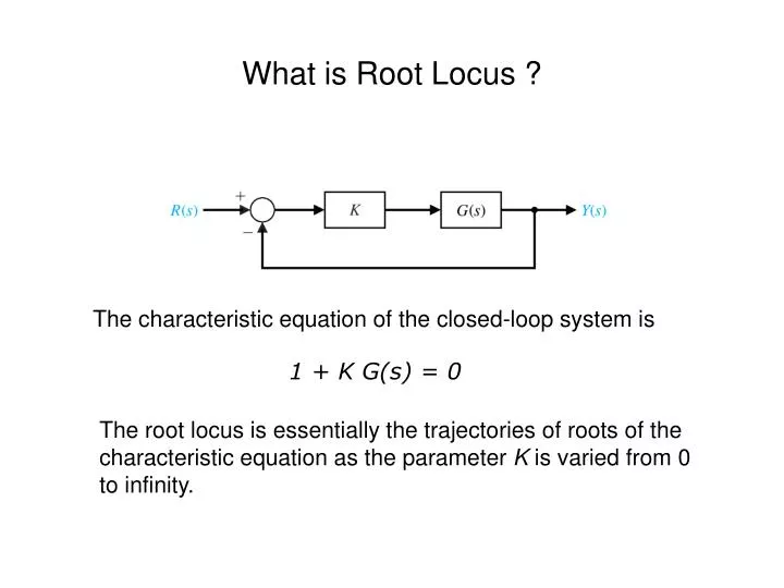
What is Root Locus ? The characteristic equation of the closed-loop system is 1 + K G(s) = 0 The root locus is essentially the trajectories of roots of the characteristic equation as the parameter K is varied from 0 to infinity.

A simple example A camera control system: How the dynamics of the camera changes as K is varied ?

A simple example (cont.) : pole locations

A simple example (cont.) : Root Locus (a) Pole plots from the table. (b) Root locus.

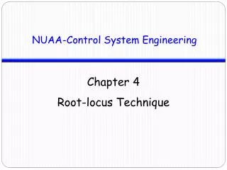
The Root Locus Method (cont.) • Consider the second-order system • The characteristic equation is:

+ y x - K>1 -2 x x K=1 K=0 K=0 K>1 S plane Introduction Characteristic equation

The Root Locus Method (cont.) • Example: • As shown below, at a root s1, the angles are:

The Root Locus Method (cont.) • The magnitude and angle requirements for the root locus are: • The magnitude requirement enables us to determine the value of K for a given root location s1. • All angles are measured in a counterclockwise direction from a horizontal line.

C R + G(s) - H(s) Root locus Open loop transfer function Closed loop transfer function The poles of the closed loop are the roots of The characteristic equation

j K= o K=0 K=0 x x  s plane K= o Root locus (Evans) • Root locus in the s plane are dependent on K • If K=0 then the roots of P(s) are those of D(s): Poles of GH(s) • If K= then the roots of P(s) are those of N(s): Zeros of GH(s) K= K=0 Open loop poles Open loop zeros

H=1 K>0 j K=1,5 K=1,5 K= K= K=0 K=0 o x o x -1  -2 Pole Zero Root locus example

Root locus example Any information from Rooth ? As K>0

Poles X O X X -2 -4 Three loci (branches) Zero Rules for plotting root loci/loca •Rule 1: Number of loci: number of poles of the open loop transfer Function (the order of the characteristic equation) •Rule 2: Each locus starts at an open-loop pole when K=0 and finishes Either at an open-loop zero or infinity when k= infinity Problem: three poles and one zero ?

K>1 -2 x x K=0 K=0 K=1 K>1 S plane Rules for plotting root loci/loca • Rule 3 Loci either move along the real axis or occur as complex Conjugate pairs of loci

K>0 j K=1,5 K=1,5 K= K= K=0 K=0 o x o x -1  -2 Pole Zero Rules for plotting root loci/loca • Rule 4 A point on the real axis is part of the locus if the number of Poles and zeros to the right of the point concerned is odd for K>0

Poles X O X X -2 -4 Three loci (branches) Zero No locus Locus on the real axis Rules for plotting root loci/loca Example

Rules for plotting root loci/loca •Rule 5: When the locus is far enough from the open-loop poles and zeros, It becomes asymptotic to lines making angles to the real axis Given by: (n poles, m zeros of open-loop) There are n-m asymptotes L=0,1,2,3…..,(n-m-1) Example

K>1 -2 x x K=0 K=0 K=1 K>1 S plane Rules for plotting root loci/loca

Rules for plotting root loci/loca • Rule 6 :Intersection of asymptotes with the real axis The asymptote intersect the real axis at a point  given by

Rules for plotting root loci/loca • Example -1 X O X X -2 -4

O X X O X Break-in Break-away O O X X Rules for plotting root loci/loca • Rule 7 The break-away point between two poles, or break-in point Between two zero  is given by: First method

-1 -2 x x x -0.423 Rules for plotting root loci/loca Example 3 asymptotes: 60 °,180 ° and 300° Part of real axis excluded Break-away point

Rules for plotting root loci/loca Second method The break-away point is found by differentiating V(s) with Respect to s and equate to zero Example

Rules for plotting root loci/loca • Rule 8: Intersection of root locus with the imaginary axis The limiting value of K for instability may be found using the Routh criterion and hence the value of the loci at the Intersection with the imaginary axis is determined Characteristic equation Example Characteristic equation

Rules for plotting root loci/loca What do we get with Routh ? If K=6 then we have an pure imaginary solution

Rules for plotting root loci/loca Example K=6 K=0 -1 -2 x x x -0.423

Rules for plotting root loci/loca • Rule 9 Tangents to complex starting pole is given by GH’ is the GH(starting p) when removing starting p Example j X -1 -j X

Rules for plotting root loci/loca • Rule 9` Tangents to complex terminal zero is given by GH’ is the GH(terminal zero) when removing terminal zero Example O j O -j

K=2 K=4 K=0 O X X -1 -2 =-3 K=2 Rules for plotting root loci/loca Example Two poles at –1 One zero at –2 One asymptote at 180° Break-in point at -3

Rules for plotting root loci/loca Example Why a circle ? Characteristic equation For K>4 For K<4 Change of origin

K=2 K=4 K=0 O X X -1 -2 =-3 K=2 Rules for plotting root loci/loca

What is Root Locus ?