Download

1 / 56
590 likes | 850 Views
The Root Locus Analysis. Eng R. L. Nkumbwa MSc, MBA, BEng, REng. Copperbelt University. Stability of Control Systems. Its all about Stability…. Auto-Pilot or Fly-by-Wire Systems.

E N D
The Root Locus Analysis Eng R. L. Nkumbwa MSc, MBA, BEng, REng. Copperbelt University
Stability of Control Systems • Its all about Stability… Eng R. L. Nkumbwa@CBU-2010
Auto-Pilot or Fly-by-Wire Systems • Let us consider the short period approximate model of the Fly Zambezi 727 aircraft landing at Lusaka International Airport. Eng R. L. Nkumbwa@CBU-2010
Auto-Pilot or Fly-by-Wire Systems • Where δe is the elevator input, • Take the output as θ, input is δe, then form the transfer function is of the form; Eng R. L. Nkumbwa@CBU-2010
Auto-Pilot or Fly-by-Wire Systems • For the Zambezi 727 (40Kft, M = 0.8) the Transfer Function reduces to: Eng R. L. Nkumbwa@CBU-2010
Auto-Pilot or Fly-by-Wire Systems • Such that, the dominant roots have a frequency of approximately 1 rad/sec and damping of about 0.4 as shown on the pole-zero map below: Eng R. L. Nkumbwa@CBU-2010
Auto-Pilot or Fly-by-Wire Systems • As the plane continue navigating the sky, we need to know and analyze where the poles are going as a function of the input command constant in the above pole-zero map. • How do we know where the poles moves as the Zambezi 727 system gain changes? • This is where Root Locus comes to address the problem and provide the solutions. Eng R. L. Nkumbwa@CBU-2010
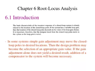
Root Locus Analysis Intro • In Control Systems I and other previous chapter, we have demonstrated the importance of the poles and zeros of the closed loop transfer function of the linear control system on the dynamic performance of the system. • The roots of the characteristic equation which are the poles of the closed loop transfer function, determine the absolute and relative stability of linear SISO Systems. Eng R. L. Nkumbwa@CBU-2010
Root Locus Analysis Intro • Another important study of the Control systems is the investigation of the trajectories of the roots of the characteristic equation or simply the Root Locus – When certain system parameters vary. • The first basic properties of the root loci and the systematic construction are due to Wade R. Evans in 1948 Eng R. L. Nkumbwa@CBU-2010
Root Locus Analysis Intro • In general, root locus may be sketched by following some simple rules and properties. • For plotting the root locus accurately the MATLAB root locus tool in the Control System Toolbox (control) or in the Time Response Analysis Tool (time tool) of ACSYS can be used. Eng R. L. Nkumbwa@CBU-2010
Root Locus Analysis Intro • The root locus technique is not confined only to the study of control systems. • In general, the method can be applied to study the behavior of roots of any algebraic equation with one or more variable parameters. Eng R. L. Nkumbwa@CBU-2010
Root Locus Example • Consider an illustrative example for the Radio Volume control in the Course Text Book by Nkumbwa on page 75. • It illustrates how root locus is applied in volume control of radio systems. Eng R. L. Nkumbwa@CBU-2010
Root Locus Example: three poles Eng R. L. Nkumbwa@CBU-2010
Root Locus Analysis Intro • General root locus is hard to determine by hand and requires Matlab tools such as: rlocus (num,den) • To obtain full result, we can get some important insights by developing a short set of plotting rules. Eng R. L. Nkumbwa@CBU-2010
Defining Root Locus • To start with, let’s make sure we’re clear on exactly what we mean by the words “Root Locus plot.” • So, what is a Root? • “A number that reduces an equation to an identity when it is substituted for one variable.” • Roots of this equation are the closed-loop poles of the feedback system. Eng R. L. Nkumbwa@CBU-2010
Defining Root Locus • Then, what is a Locus? • “The set of all points whose location is determined by stated conditions.” • The “stated conditions” here are that 1 + kL (s) = 0 for some value of k, and the “points” whose 0 locations matter to us are points in the s-plane. Eng R. L. Nkumbwa@CBU-2010
Defining Root Locus • Now, what is a Root Locus? • The set of all points in the s-plane that satisfy the equation 1 + kL (s) = 0 for some 0 value of k. • Root locus is a graphical presentation of the closed- loop poles as a system parameter is varied. • Root locus is a powerful method of analysis and design for stability and transient response. Eng R. L. Nkumbwa@CBU-2010
Defining Root Locus • The root- locus technique is a graphical method for sketching the locus of the roots in the s-plane as a parameter is varied. • In fact, the root- locus method provides the engineer with a measure of the sensitivity of the roots of the system to a variation in the parameter being considered. Eng R. L. Nkumbwa@CBU-2010
Some Root Locus Basic Questions • What points are on the root locus? • Where does the root locus start? • Where does the root locus end? • When/where is the locus on the real line? • Etc • Answering these and many more questions will help us understand Root Locus technique. Eng R. L. Nkumbwa@CBU-2010
Pole and Zero Locations by R-Locus • Let's say we have a closed-loop transfer function for a particular system: Eng R. L. Nkumbwa@CBU-2010
Pole and Zero Locations by R-Locus • Where N is the numerator polynomial and D is the denominator polynomial of the transfer functions, respectively. • Now, we know that to find the poles of the equation, we must set the denominator to 0, and solve the characteristic equation. Eng R. L. Nkumbwa@CBU-2010
Pole and Zero Locations by R-Locus • In other words, the locations of the poles of a specific equation must satisfy the following relationship: Eng R. L. Nkumbwa@CBU-2010
Pole and Zero Locations by R-Locus • And from the above equation we can manipulate an equation such as: Eng R. L. Nkumbwa@CBU-2010
Pole and Zero Locations by R-Locus • And finally by converting to polar coordinates, we get: Eng R. L. Nkumbwa@CBU-2010
Equation for all Gain Values • Now we have 2 equations that govern the locations of the poles of a system for all gain values: • The Magnitude Equation Eng R. L. Nkumbwa@CBU-2010
Equation for all Gain Values • The Angle Equation Eng R. L. Nkumbwa@CBU-2010
Root-Locus Design Procedure • In laplace transform domain, when the gain is small the poles start at the poles of the open loop transfer function. • When gain becomes infinity, the poles move to overlap the zeros of the system. • This means that on a root-locus graph, all the poles move towards a zero. Eng R. L. Nkumbwa@CBU-2010
Root-Locus Design Procedure • Only one pole may move towards one zero and this means that there must be the same number of poles as zeros. • If there are fewer zeros than poles in the transfer function, there are a number of implicit zeros located at infinity that the poles will approach. Eng R. L. Nkumbwa@CBU-2010
Note • Remember that, Poles are marked on the graph with an 'X' and zeros are marked with an 'O‘ by common convention. Eng R. L. Nkumbwa@CBU-2010
Root-Locus Design Procedure • We can start drawing the root-locus by first placing the roots of b(s) on the graph with an 'X'. • Next, we place the roots of a(s) on the graph, and mark them with an 'O'. • Where b(s) and a(s) are the numerator and denominator of the system transfer function. Eng R. L. Nkumbwa@CBU-2010
Root-Locus Design Procedure • Next, we examine the real-axis. • Starting from the right-hand side of the graph and traveling to the left, we draw a root-locus line on the real-axis at every point to the left of an odd number of poles on the real-axis. Eng R. L. Nkumbwa@CBU-2010
Root-Locus Design Procedure • Now, a root-locus line starts at every pole. • Therefore, any place that two poles appear to be connected by a root locus line on the real-axis, the two poles actually move towards each other, and then they "breakaway", and move off the axis. • The point where the poles break off the axis is called the breakaway point. Eng R. L. Nkumbwa@CBU-2010
Note • It is important to note that the s-plane is symmetrical about the real axis, so whatever is drawn on the top half of the S-plane, must be drawn in mirror-image on the bottom-half plane. Eng R. L. Nkumbwa@CBU-2010
Root-Locus Design Procedure • Once a pole breaks away from the real axis, they can either travel out towards infinity (to meet an implicit zero) or they can travel to meet an explicit zero, or they can re-join the real-axis to meet a zero that is located on the real-axis. Eng R. L. Nkumbwa@CBU-2010
Root-Locus Design Procedure • If a pole is traveling towards infinity, it always follows an asymptote. • The number of asymptotes is equal to the number of implicit zeros at infinity. Eng R. L. Nkumbwa@CBU-2010
Root-Locus Construction Rules • Rule 1: Starting Point (K=0) • The root locus starts at open loop poles. Or there is one branch of the root-locus for every root of b(s). • Rule 2: Terminating Point (K=infinity) • The root locus terminates at open loop zeros which include those at infinity. • Rule 3: Number of Distinct Root Loci • There will be as many root loci as the highest number of finite open loop poles or zeros. Eng R. L. Nkumbwa@CBU-2010
Root-Locus Construction Rules • Rule 4: Symmetry of the Root Loci • The root loci are symmetrical with respect to the real axis and all complex roots are conjugate. • Rule 5: Angle of Asymptotes • The root loci are asymptotic to straight lines at large values and the angle of asymptotes is given by Eng R. L. Nkumbwa@CBU-2010
Root-Locus Construction Rules • Rule 6: Asymptotic Intersection • The asymptotes intersects the real axis at the point given by Eng R. L. Nkumbwa@CBU-2010
Root-Locus Construction Rules • Rule 7: Root Locus Location on the Real Axis • The root loci may be found on portions of the real axis to the left of an old number of open loop poles and zeros. • Rule 8: Locus Breakaway Point • The points at which the root locus break away can be calculated by the following: Eng R. L. Nkumbwa@CBU-2010
Root-Locus Construction Rules • Rule 9: Angle of Departure and Arrival • Find the formula • Rule 10: Point of Intersection with the Imaginary Axis • Find the formula • Rule 11: Determination of K • Find the formula • And many more rules and equations Eng R. L. Nkumbwa@CBU-2010
Root Locus Example • A single- loop feedback system has a characteristic equation as follows: Eng R. L. Nkumbwa@CBU-2010
Root Locus Example • We wish to sketch the root locus in order to determine the effect of the gain K. The poles and the zeros are located in the s-plane as: Eng R. L. Nkumbwa@CBU-2010
Root Locus Example Eng R. L. Nkumbwa@CBU-2010
Root Locus Example • The root loci on the real axis must be located to the left of an odd number of poles and zeros and are therefore located as shown on the figure above in heavy lines. Eng R. L. Nkumbwa@CBU-2010
Root Locus Example • The intersection of the asymptotes is: Eng R. L. Nkumbwa@CBU-2010
Root Locus Example • The angles of the asymptotes are: Eng R. L. Nkumbwa@CBU-2010
Root Locus Example • There are three asymptotes, since the number of poles minus the number of zeros, n – m = 3. • Also, we note that the root loci must begin at poles, and therefore two loci must leave the double pole at s = - 4. Then, with the asymptotes as sketched below, we may sketch the form of the root locus: Eng R. L. Nkumbwa@CBU-2010
Root Locus Example Eng R. L. Nkumbwa@CBU-2010