Download
1 / 74
740 likes | 829 Views
Advanced Design Methods -Optimization of Design Meng Xianyi Prof. Ph.D Department of Mechanical and Electronic Engineering Beijing Institute of Civil Engineering and Architecture. Objective

E N D
Advanced Design Methods -Optimization of Design Meng Xianyi Prof. Ph.D Department of Mechanical and Electronic Engineering Beijing Institute of Civil Engineering and Architecture
Objective Students could understand about opt, create mathematical model and solve simple problem by using computer after learning this chapter. Chapter Objective Lesson 1 3.1 General Description** 1.Background 2.Differences? Examples 3.1 To design a bracket Examples 3.1 To design a Column Lesson 2 3.2 Mathematical model for optimization of design *** 3.2.1 Design variables and design domain 1)Design variables 2)Design domain 3.2.2 Constraints 3.3.3 objective function Lesson Objectives
3.2.4 Mathematical model for optimization of design Example 3.3 Lesson 3 3.3 Numerical solution of mathematical model** 3.4 one dimensional search method* 3.4.1 Advancing and Retreating Method* Lesson 4 3.4.2 Golden Section Method* Principle* Procedures 3.5 multi - dimensional optimization method** General description Lesson 5 Gradient method* Lesson Objectives
3.6 Penalty function method** Description Example 3.7* Solution Example 3.5** Exercise** Lesson 6 3.6.1 Inner point method** Characteristics 3.6.2 Outer point method** 3.6.3 Summery of SUMT** 3.6.4 Discussion of SUMT** 3.7 Application example** Example 3.6 Solution Lesson 7, 8, 9 Computing and examination *** Lesson Objectives
Chapter 3Optimization of Design 3.1 General Description 1.Background • To make something best Such as • Ordinary and optimal design • Developed for 20 years Math programming + computer BICEA JDX Meng Xianyi 2005
2.Differences? • Automatically adjusting • Using Computer 3.What included? • Build Model Mechanical engineering area • Solving BICEA JDX Meng Xianyi 2005
Examples 3.1 To design a bracket D---outer diameter d---inner diameter F---external force b---thickness H---height F H b d D BICEA JDX Meng Xianyi 2005
Examples 3.1 • There are a group of different values of the parameters • Decide the sizes of D, d, H and b to make the bracket lightest BICEA JDX Meng Xianyi 2005
Examples 3.2 To design a Column F---force 22680 N L---length 254 cm E---Young’s module 7.03e4 MPa ---Material density 2.768e-6 g/cm3 t---thickness D0---outer diameter D1---inner diameter t F D0 D1 L BICEA JDX Meng Xianyi 2005
Solution Let D=(D0+D1)/2 Weight: S.t. 1.stability where 2.strength 3.technical & geometrical BICEA JDX Meng Xianyi 2005
D=8.9 σ- σc=0 t/cm Acceptable area m=2.722kg Line of constant m m=1.814kg [σ] =140MPa t=0.1 σ– [σ ]=0 0 8.128 D/cm
3.2 Mathematical model for optimization of design 3.2.1 Design variables and design domain 1)Design variables • Design parameters • Defined in the design • Independent each other Examples: dimension sizes, length, coordinates, material, temperature , etc. BICEA JDX Meng Xianyi 2005
2)Design domain All design variables make up a design domain X=[x1 x2…xn] 3-dimension design space x2 x1 x3 BICEA JDX Meng Xianyi 2005
3.2.2 Constraints Limits: strength limit, stiffness requirement, frequency …, etc. gi(X) =σ- [σ] ≤0 ( inequality ) (i=1,2,3…m) hj(X)=0 ( equality ) (j=1,2,3…p<n, n---number of variables) BICEA JDX Meng Xianyi 2005
3.3.3 objective function Criterion to be used to judge if a design is the best or not. Such as weight, volume, cost, speed, etc. F(X)= Where D=x1 t =x2 BICEA JDX Meng Xianyi 2005
3.2.4 Mathematical model for optimization of design Includes: design variables, constraint conditions, objective function min f(X) x Rn s.t. gi(X)≤0 (i=1,2,3…m) hj(X)=0 (j=1,2,3…p<n) BICEA JDX Meng Xianyi 2005
Example 3.3 Given Producing two kinds of products: Product A Product B BICEA JDX Meng Xianyi 2005
Question: To make the profits most, how many quantities of each product made everyday? Solution: A—x1, B---x2 F(x1 ,x2)=60x1+120 x2 BICEA JDX Meng Xianyi 2005
g1(X)=9x1+4x2 g2(X)=3x1+10x2 g3(X)=4x1+5x2 BICEA JDX Meng Xianyi 2005
Seek x1, x2 To make -F(x1 ,x2)=-(60x1+120 x2)min s.t. g1(X)=9x1+4x2 ≤360 g2(X)=3x1+10x2 ≤300 g3(X)=4x1+5x2 ≤200 g3(X)=-x1 ≤0 g3(X)=-x2 ≤0 BICEA JDX Meng Xianyi 2005
3.3 Numerical solution of mathematical model • Theoretical solution • Numerical iteration algorithm • Accurate X(0) , X(1) ,…X(k) , X(k+1),… f(X(0) )> f(X(1) )>… f(X(k) )> f(X(k+1) )>… X*=LimX(k) k ∞ BICEA JDX Meng Xianyi 2005
Approximate If | X(k) - X(k+1) | ≤ε Let X*= X(k+1) Iteration formula X(k+1) = X(k) +αS(k) X(k) ---current point X(k+1) ---next point α--- increment factor S(k) ---direction BICEA JDX Meng Xianyi 2005
D=8.9 S(0) α0 σ- σc=0 X(0) t/cm X(1) X(2) Acceptable area X(3) m=2.722kg m=1.814kg σ=140MPa t=0.1 X* 0 8.128 D/cm
The iteration steps 1)Difine an initial point X(0)and the convergence errorε 2)Difine a searching direction S(0) 3)Choose an increment factorαk 4)Convergence judging BICEA JDX Meng Xianyi 2005
If X(k+1) meet the convergence requirement, terminate Otherwise go to 2), Continue for a new point Convergence error • | X(k+1) - X(k) | ≤ ε BICEA JDX Meng Xianyi 2005
3.4 one dimensional search method Description: To determining increment factor αk • Two steps: 1) define initial interval • 2) shrink the interval get the extremum point • 3.4.1 Advancing and Retreating Method– • to define initial interval • Two requirements • Exrtremum point existing • Single peak BICEA JDX Meng Xianyi 2005
Advancing retreating f1 f4 f1 f2 f2 f3 f3 f4 x4 x2 x3 x1 in –h,-2h,-4h… f2 > f3 < f4, high-low-high, [x2, x4]----[A, B] In h,2h,4h… f2 > f3 < f4, high-low-high, [x2, x4]----[A, B] BICEA JDX Meng Xianyi 2005
Definex0,h Let x1=x0,f1=f(x0) X2=x0+h,f2=f(x2) f1>f2? h=-h N Y X3=x1,f3=f1 X1=x2,f1=f2 x2=x3,f2=f3 h=2h X1=x2,f1=f2 X2=x3,f2=f3 x3=x0+h,f3=f(x3) N f2<f3? h=2h
Y c=x2,fc=f2 h>0? Y N a=x1,fa=f1 b=x3,fb=f3 a=x3,fa=f3 b=x1,fb=f1 Obtain a,b,c,fa,fb,fc Exit
3.4.2 Golden Section Method To find the extremum point by shrinking the interval One of many methods Principal general methods: • Inserting two points • Comparing the values of functions of the two points • Shrink the interval by giving up the segment which… • If interval less than a convergence, stop Many different ways according to the inserting way of the two points BICEA JDX Meng Xianyi 2005
f1 f2 f1 f2 b a b a f1<f2 f1>f2 BICEA JDX Meng Xianyi 2005
principle 1-λ 1 X1=a+(1-λ)(b-a) X2=a+ λ(b-a) λ x1 x2 λ (1-λ)/λ = λ λ2 = (1-λ) λ≈0.618 0.382 /0.618=0.618 1 If f2>f1 λ x1 x2 BICEA JDX Meng Xianyi 2005
If f1 > f2 1-λ 1 λ x1 x2 λ 1 λ x1 x2 BICEA JDX Meng Xianyi 2005
Shrink λ one step , step number n 0.618n(b-a)≤ ε n ≥ ln(ε/(b-a))/ln0.618 BICEA JDX Meng Xianyi 2005
procedures 1)Define an interval [a,b] and a convergence accuracy 2)Decide the inserting points and calculate the corresponding function values X1 = a + 0.382(b-a), f1=f(x1) X2 = a + 0.618(b-a), f2=f(x2) 3)Compare the two function values 4)Convergence judging 5)Make new inserting points, and repeat the above steps BICEA JDX Meng Xianyi 2005
Define a0,b0, a=a0,b=b0 x1=a+0.382(b-a),f1=f(x1) x2=a+0.618(b-a),f2=f(x2) N Y f1<f2? N0=1 N0=0 a=x1 x1=x2,f1=f2 b=x2 x2=x1,f2=f1 Y N ︴b-a︴≤ ε Y N N0=0? x*=(a+b)\2 x1=a+0.382(b-a) f1=f(x1) x2=a+0.618(b-a) f2=f(x2) Exit
Example 3.4 Question: Solution: (1)Define initial interval (2)Shrink the interval by GSM 1)The first time of shrink interval 2)The second time 3)The third time 4)The fourth time BICEA JDX Meng Xianyi 2005
5)The fifth time BICEA JDX Meng Xianyi 2005
3.5 multi - dimensional optimization method General description min f(X) x Rn s.t. gj(X)≤0 (j=1,2,…,m) hv(X)=0 (v=1,2,…,p<n) Two categories: • Derivative method---using first or second derivatives of objective function • Module method---comparing points’ function values Advantages and disadvantages BICEA JDX Meng Xianyi 2005
Another classifying type Direct method and indirect method 1.Direct method: Iteration within the domain directly 2.Indirect method: • Iteration without constraints • Problem with constraints is transformed to those without constraints Introduce gradient method BICEA JDX Meng Xianyi 2005
Gradient method Iteration direction---negative gradient Since then BICEA JDX Meng Xianyi 2005
derivative formula get BICEA JDX Meng Xianyi 2005
S(7) S(3) S(5) S(1) S(6) X(6) X(7) X(4) S(4) X(5) X(2) S(2) X(3) X(0) S(0) X(1) BICEA JDX Meng Xianyi 2005
Procedures: 1)Define initial point 2)Calculate gradient, construct searching Direction 3)Conduct one dimensional searching and get new point BICEA JDX Meng Xianyi 2005
4) Convergence judging Let If satisfied, otherwise go to 2) continue BICEA JDX Meng Xianyi 2005
3.6 Penalty function method Description: • Constrained opt---unconstrained opt • Sequential Unconstrained Minimization Technique---SUMT • Get penalty when approaching the boundary BICEA JDX Meng Xianyi 2005
d1 d2 d2 G FR FR L\2 L\2 L L L L Example 3.7 Question Axle rotating with a speed of ω Condition Natural frequency> rotating speed Requirement lightest m ω BICEA JDX Meng Xianyi 2005
solution Objective Constraint ωk=k ω ω k---natural frequency ω k=√g/δ g---acceleration of gravity δ---static deformation δ=10.67Gl3 [1/d14+2.38/d24] /Eπ k---coefficient >1 BICEA JDX Meng Xianyi 2005
G---weight of the plate, E---Young’s module After Substituting, the constraint: 1/d14+2.38/d24-c=0 where c=πEg/ 10.67Gl3 ω2k2 BICEA JDX Meng Xianyi 2005
Model Seek x=[x1, x2]T To make f(x)=2x12+x22 min s.t. 1/x14+2.38/x24-c=0 c=πEg/ 10.67Gl3 ω2k2 BICEA JDX Meng Xianyi 2005