Download
1 / 44
440 likes | 599 Views
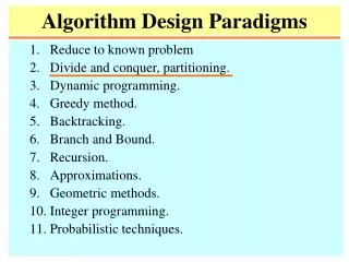
Algorithm Design Methods. Spring 2007 CSE, POSTECH. Algorithm Design Methods. Greedy method Divide and conquer Dynamic programming Backtracking Branch and bound. Some Methods Not Covered. Linear Programming Integer programming Simulated annealing Neural networks Genetic algorithms

E N D
Algorithm Design Methods Spring 2007 CSE, POSTECH
Algorithm Design Methods • Greedy method • Divide and conquer • Dynamic programming • Backtracking • Branch and bound
Some Methods Not Covered • Linear Programming • Integer programming • Simulated annealing • Neural networks • Genetic algorithms • Tabu search
Optimization Problem • A problem in which some function(called the optimization/objective function)is to be optimized (usually minimized or maximized) • It is subject to some constraints.
Machine Scheduling • Find a schedule that minimizes the finish time. • optimization function … finish time • constraints • Each job is scheduled continuously on a single machine for an amount of time equal to its processing requirement. • No machine processes more than one job at a time.
Bin Packing • Pack items into bins using fewest number of bins. • optimization function … number of bins • constraints • Each item is packed into a single bin. • The capacity of no bin is exceeded.
Min Cost Spanning Tree • Find a spanning tree that has minimum cost. • optimization function … sum of edge costs • constraints • Must select n-1 edges of the given n vertex graph. • The selected edges must form a tree.
Feasible and Optimal Solutions • A feasible solution is a solution that satisfies the constraints. • An optimal solution is a feasible solution that optimizes the objective/optimization function.
Greedy Method • Solve problem by making a sequence of decisions. • Decisions are made one by one in some order. • Each decision is made using a greedy criterion. • A decision, once made, is (usually) not changed later.
Machine Scheduling LPT Scheduling. • Schedule jobs one by one in decreasing order of processing time (i.e., longest processing time first). • Each job is scheduled on the machine on which it finishes earliest. • Scheduling decisions are made serially using a greedy criterion (minimize finish time of this job). • LPT scheduling is an application of the greedy method.
LPT Schedule • LPT rule does not guarantee minimum finish time schedules. (LPT Finish Time)/(Minimum Finish Time) <= 4/3 – 1/(3m) where m is number of machines. • Minimum finish time scheduling is NP-hard. • In this case, the greedy method does not work. • Greedy method does, however, give us a good heuristic for machine scheduling.
Container Loading Problem • Ship has capacity c. • m containers are available for loading. • Weight of container i is wi. • Each weight is a positive number. • Sum of container weight < c. • Load as many containers as possible without sinking the ship.
Greedy Solution • Load containers in increasing order of weight until we get to a container that does not fit. • Does this greedy algorithm always load the maximum number of containers? • Yes. May be proved using a proof by induction.(see Theorem 13.1, p. 624 of text.)
Container Loading with 2 Ships • Can all containers be loaded into 2 ships whose capacity is c each? • Same as bin packing with 2 bins(Are 2 bins sufficient for all items?) • Same as machine scheduling with 2 machines(Can all jobs be completed by 2 machines in c time units?) • NP-hard
0/1 Knapsack Problem • Hiker wishes to take n items on a trip. • The weight of item i is wi. • The knapsack has a weight capacity c. • If sum of items weights <= c,all n items can be carried in the knapsack. • If sum of item weights > c,some items must be left behind. • Which items should be taken out?
0/1 Knapsack Problem • Hiker assigns a profit/value pi to item i. • All weights and profits are positive numbers. • Hiker wants to select a subset of n items to take. • The weight of the subset should not exceed the capacity of the knapsack. (constraint) • Cannot select a fraction of an item. (constraint) • The profit/value of the subset is the sum of the profits of the selected items. (optimization function) • The profit/value of the selected subset should be maximum. (optimization criterion)
0/1 Knapsack Problem • Let xi=1 when item i is selected andlet xi=0 when item i is not selected. maximize Sigma(i=1…n) pixi subject to Sigma(i=1…n) wixi <= c • See the formula and constraints on page 625
Greedy Attempt 1 • Be greedy on capacity utilization(select items in increasing order of weights). • n = 2, c = 7 • w = [3, 6] • p = [2, 10] • Only 1 item is selected, x = [1, 0].Profit/value of selection is 2.It is not the best selection.
Greedy Attempt 2 • Be greedy on profit earned(select items in decreasing order of profit). • n = 3, c = 7 • w = [7, 3, 2] • p = [10, 8, 6] • Only 1 item is selected , x = [1, 0, 0].Profit/value of selection is 10.It is not the best selection.
Greedy Attempt 3 • Be greedy on profit density (p/w)(select items in decreasing order of profit density). • n = 2, c = 7 • w = [1, 7] • p = [10, 20] • Only 1 item is selected, x = [1, 0].Profit/value of selection is 10.It is not the best selection.
Greedy Attempt 4 • Select a subset with <= k items. • If the weight of this subset is > c,discard the subset. • If the subset weight is <= c,fill as much of the remaining capacity as possible by being greedy on profit density. • Try all subsets with <= k items andselect the one that yields maximum profit.
Chapter 14: Divide and Conquer • A large problem is solved as follows: • Divide the large problem into smaller problems. • Solve the smaller problems somehow. • Combine the results of the smaller problemsto obtain the result for the original large problem. • A small problem is solved in some other way.
Small and Large Problem • Small problem • Sort a list that has n <= 10 elements. • Find the minimum of n <= 2 elements. • Large problem • Sort a list that has n > 10 elements. • Find the minimum of n > 2 elements.
Solving a Small Problem • A small problem is solvedusing some direct/simple strategy. • Sort a list that has n <= 10 elements.Use insertion, bubble, or selection sort. • Find the minimum of n <= 2 elements.When n = 0, there is no minimum element.When n = 1, the single element is the minimum.When n = 2, compare the two elements and determine which is smaller.
Sort a Large List • Sort a list that has n > 10 elements. • Sort 15 elements by dividing them into 2 smaller lists.One list has 7 elements and the other has 8 elements. • Sort these two lists using the method for small lists. • Merge the two sorted lists into a single sorted list.
Find the Min of a Large List • Find the minimum of 20 elements. • Divide into two groups of 10 elements each. • Find the minimum element in each group somehow. • Compare the minimums of each group to determine the overall minimum.
Recursion In Divide and Conquer • Often the smaller problems that result from the divide step are instances of the original problem(true for our sort and min problems). In this case, • If the new problem is a smaller problem,it is solved using the method for small problems. • If the new problem is a large instance, it is solvedusing the divide-and-conquer method recursively. • Generally, performance is best when the smaller problems that result from the divide step are of approximately the same size.
Recursive Find Min • Find the minimum of 20 elements. • Divide into two groups of 10 elements each. • Find the minimum element in each group recursively.The recursion terminates when the number of elementsis <= 2. At this time the minimum is found using the method for small problems. • Compare the minimums of each group to determine the overall minimum.
Merge Sort – another Divide & Conquer Example • Sort the first half of the array using merge sort. • Sort the second half of the array using merge sort. • Merge the first half of the array with the second half.
Merge Sort Algorithm • Merge is an operation that combines two sorted arrays. • Assume the result is to be placed in a separate array called result (already allocated). • The two given arrays are called front and back. • front and back are in increasing order. • For the complexity analysis,the size of the input, n, is the sum nfront + nback.
Merge Sort Algorithm • For each array keep track of the current position. • REPEAT until all the elements of one of the given arrays have been copied into result: • Compare the current elements of front and back. • Copy the smaller into the current position of result (break the ties however you like). • Increment the current position of result and the array that was copied from. • Copy all the remaining elements of the other given array into result.
Merge Sort Algorithm - Complexity • Every element in front and back is copied exactly once. Each copy is two accesses, so the total number of accessing due to copying is 2n. • The number of comparisons could beas small as min(nfront, nback) or as large as n-1.Each comparison is two accesses.
Merge Sort Algorithm - Complexity • In the worst casethe total number of accesses is2n +2(n-1) =O(n). • In the best casethe total number of accesses is2n + 2min(nfront,nback) = O(n). • The average case is between the worst and best case and is therefore also O(n).
Merge Sort Algorithm • Split anArray into two non-empty parts anyway you like. For example,front = the first n/2 elements in anArrayback = the remaining elements in anArray • Sort front and back by recursively calling MergeSort. • Now you have two sorted arrays containing all the elements from the original array.Use merge to combine them, put the result in anArray.
0~6 0~2 3~6 0~0 1~2 3~4 5~6 1~1 2~2 3~3 4~4 5~5 6~6 MergeSort Call Graph (n=7) • Each box represents one invocation of MergeSort. • How many levels are there in generalif the array is divided in half each time?
n n/2 n/2 n/4 n/4 n/4 n/4 1 1 1 1 1 1 1 1 MergeSort Call Graph (general) • Suppose n = 2k. How many levels? • How many boxes on level j? • What values is in each box at level j?
Quick Sort • Quicksort can be seen as a variation of mergesort in which front and back are defined in a different way.
Quicksort Algorithm • Partition anArray into two non-empty parts. • Pick any value in the array, pivot. • small = the elements in anArray< pivot • large = the elements in anArray> pivot • Place pivot in either part,so as to make sure neither part is empty. • Sort small and large by recursively calling QuickSort. • How would you merge the two arrays? • You could use merge to combine them, but because the elements in small are smaller than elements in large, simply concatenatesmall and large, and put the result into anArray.
Quicksort: Complexity Analysis • Like mergesort,a single invocation of quicksort on an array of size phas complexity O(p): • p comparisons = 2*p accesses • 2*p moves (copying) = 4*p accesses • Best case: every pivot chosen by quicksort partitions the array into equal-sized parts. In this case quicksort is the same big-O complexity as mergesort – O(n log n)
n 1 n-1 1 n-2 1 1 Quicksort: Complexity Analysis • What would be the worst case scenario? • Worst case: the pivot chosen is the largest or smallest value in the array. Partition creates one part of size 1 (containing only the pivot), the other of size p-1.
Quicksort: Complexity Analysis Worst case: • There are n-1 invocations of quicksort (not counting base cases) with arrays of size:p = n, n-1, n-2, …, 2 • Since each of these does O(p),the total number of accesses isO(n) + O(n-1) + … + O(1) = O(n2) • Ironically the worst case occurs when the list is sorted (or near sorted)!
Quicksort: Complexity Analysis • The average case must be betweenthe best case O(n log n) and the worst case is O(n2). • Analysis yields a complex recurrence relation. • The average case number of comparisons turns out to be approximately 1.386*n*log n – 2.846*n. • Therefore the average case time complexity isO(n log n).
Quicksort: Complexity Analysis • Best case O(n log n) • Worst case O(n2) • Average case O(n log n) • Note that the quick sort is inferior to insertion sort and merge sort if the list is sorted, nearly sorted, or reverse sorted.
READING • READ Chapter 13 & 14 • Chapters 15 (Dynamic Programming), 16 (Backtracking) and 17 (Branch and Bound) are useful algorithm design methods and you should read and try to understand them • The final exam will mostly cover (about 90%) from the second half materials