Download
1 / 34
360 likes | 576 Views
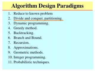
Algorithm Design Methods. Greedy method. Divide and conquer. Dynamic Programming. Backtracking. Branch and bound. Some Methods Not Covered. Linear Programming. Integer Programming. Simulated Annealing. Neural Networks. Genetic Algorithms. Tabu Search. Optimization Problem.

E N D
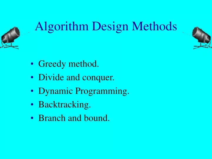
Algorithm Design Methods Greedy method. Divide and conquer. Dynamic Programming. Backtracking. Branch and bound.
Some Methods Not Covered • Linear Programming. • Integer Programming. • Simulated Annealing. • Neural Networks. • Genetic Algorithms. • Tabu Search.
Optimization Problem A problem in which some function (called the optimization or objective function) is to be optimized (usually minimized or maximized) subject to some constraints.
Machine Scheduling Find a schedule that minimizes the finish time. • optimization function … finish time • constraints • each job is scheduled continuously on a single machine for an amount of time equal to its processing requirement • no machine processes more than one job at a time
Bin Packing Pack items into bins using the fewest number of bins. • optimization function … number of bins • constraints • each item is packed into a single bin • the capacity of no bin is exceeded
Min Cost Spanning Tree Find a spanning tree that has minimum cost. • optimization function … sum of edge costs • constraints • must select n-1edges of the given n vertex graph • the selected edges must form a tree
Feasible And Optimal Solutions A feasible solution is a solution that satisfies the constraints. An optimal solution is a feasible solution that optimizes the objective/optimization function.
Greedy Method • Solve problem by making a sequence of decisions. • Decisions are made one by one in some order. • Each decision is made using a greedy criterion. • A decision, once made, is (usually) not changed later.
Machine Scheduling LPT Scheduling. Schedule jobs one by one and in decreasing order of processing time. Each job is scheduled on the machine on which it finishes earliest. Scheduling decisions are made serially using a greedy criterion (minimize finish time of this job). LPT scheduling is an application of the greedy method.
Machine Scheduling • Greedy solution: • Assign tasks in stages, one task per stage • assign in nondecreasing order of task start times. • Call a machine old if at least one task has been assigned to it. Otherwise is new. • Greedy Criterion: minimize the length of the schedule constructed so far, or: If an old machine becomes available by the start time of the task to be assigned, assign the task to this machine; if not assign it to a new machine.
Machine Scheduling Example • Tasks in nondecreasing order: a, f, b, c, g, e, d • Algorithm has 7 stages. • Stage 1: no old machines, so assign a to a new machine (M1). M1 busy from time 0 to 2. • Stage 2: task f assigned to new machine (M2). • Stage 3: task b assigned to M1. M1 busy till time 7 • Stage 4: c assigned to new machine • etc. See diagram.
LPT Schedule LPT rule does not guarantee minimum finish time schedules. (LPT Finish Time)/(Minimum Finish Time) <= 4/3 - 1/(3m) where m is number of machines Minimum finish time scheduling is NP-hard. In this case, the greedy method does not work. Greedy method does, however, give us a good heuristic for machine scheduling.
LPT Schedule Time: O(n log2n) if use a O(n log2n) sorting algorithm.
Container Loading • Ship has capacity c. • m containers are available for loading. • Weight of container i is wi. • Each weight is a positive number. • Sum of container weights > c. • Load as many containers as is possible without sinking the ship.
Greedy Solution • Load containers in increasing order of weight until we get to a container that doesn’t fit. • Does this greedy algorithm always load the maximum number of containers? • Yes. May be proved using a proof by induction (see later).
Greedy Solution Example • n = 8, c=400 [w1,w2,…,w8]=[100,200,50,90,150,50,20,80] • consider containers in order 7,3,6,8,4,1,5,2 • Containers 7,3,6,8,4,1 together weigh 390 units • Available capacity is 10 units, not enough for any more. • Greedy solution: [x1,…,x8]=[1,0,1,1,0,1,1,1] and
Container Loading With 2 Ships Can all containers be loaded into 2 ships whose capacity is c (each)? • Same as bin packing with 2 bins. • Are 2 bins sufficient for all items? • Same as machine scheduling with 2 machines. • Can all jobs be completed by 2 machines in c time units? • NP-hard.
0/1 Knapsack Problem • Hiker wishes to take nitems on a trip. • The weight of item i is wi. • The items are to be carried in a knapsack whose weight capacity is c. • When sum of item weights <= c, all n items can be carried in the knapsack. • When sum of item weights > c, some items must be left behind. • Which items should be taken/left?
0/1 Knapsack Problem • Hiker assigns a profit/value pi to item i. • All weights and profits are positive numbers. • Hiker wants to select a subset of the n items to take. • The weight of the subset should not exceed the capacity of the knapsack. (constraint) • Cannot select a fraction of an item. (constraint) • The profit/value of the subset is the sum of the profits of the selected items. (optimization function) • The profit/value of the selected subset should be maximum. (optimization criterion)
n pi xi maximize i = 1 n wi xi <= c subject to i = 1 0/1 Knapsack Problem Let xi = 1 when item i is selected and let xi = 0 when item i is not selected. and xi = 0 or 1 for all i
Greedy Attempt 1 Be greedy on capacity utilization. • Select items in increasing order of weight. n = 2, c = 7 w = [3, 6] p = [2, 10] only item 1 is selected profit/value of selection is 2 not best selection!
Greedy Attempt 2 Be greedy on profit earned. • Select items in decreasing order of profit. n = 3, c = 7 w = [7, 3, 2] p = [10, 8, 6] only item 1 is selected profit/value of selection is 10 not best selection!
Greedy Attempt 3 Be greedy on profit density (p/w). • Select items in decreasing order of profit density. n = 2, c = 7 w = [1, 7] p = [10, 20] only item 1 is selected profit/value of selection is 10 not best selection!
Greedy Attempt 3 Be greedy on profit density (p/w). • Works when selecting a fraction of an item is permitted • Select items in decreasing order of profit density, if next item doesn’t fit take a fraction so as to fill knapsack. n = 2, c = 7 w = [1, 7] p = [10, 20] item 1 and 6/7 of item 2 areselected
0/1 Knapsack Greedy Heuristics • Select a subset with <= k items. • If the weight of this subset is > c, discard the subset. • If the subset weight is <= c, fill as much of the remaining capacity as possible by being greedy on profit density. • Try all subsets with <= k items and select the one that yields maximum profit.
0/1 Knapsack Greedy HeuristicsExample • n = 4, w = [2,4,6,7], p = [6,10,12,13], c=11 • when k = 0 fill knapsack in nonincreasing order of profit density. • place object 1, then object 2. • total weight = 6; remaining weight = 5. • So solution is x = [1,1,0,0,0] • solution profit is 16
0/1 Knapsack Greedy HeuristicsExample • n = 4, w = [2,4,6,7], p = [6,10,12,13], c=11 • now let k = 1. subsets are {1},{2},{3},{4} • Subsets {1} and {2} lead to same solution as when k = 0. Why? • Consider subset {3}. Set x3 = 1. • 5 units of capacity remain. So consider objects in nonincreasing order of profit density. • So consider object 1 first. It fits, x1 = 1. • 3 units of capacity left; nothing fits. • Solution is x = [1,0,1,0], Profit = 18. • Subset {4} gives solution x = [1,0,0,1] and profit 19. Best solution so far.
0/1 Knapsack Greedy HeuristicsExample • n = 4, w = [2,4,6,7], p = [6,10,12,13], c=11 • now let k = 2. Must consider previous subsets and the subsets {1,2},{1,3},{1,4},{2,3},{2,4},{3,4} • Subset {3,4} is infeasible and is discarded. Why? • Subset {1,2} gives x = [1,1,0,0] with profit = 16 • Subset {1,3} gives x = [1,0,1,0] with profit = 18 • Subset {1,4} gives x = [1,0,0,1] with profit = 19 • Subset {2,3} gives x = [0,1,1,0] with profit = 22 • Subset {2,4} gives x = [0,1,0,1] with profit = 23 • Subset {3,4} gives x = [0,0,1,1] with profit = 25 • So the solution for k <= 2 is {3,4} with profit = 25
0/1 Knapsack Greedy Heuristics • Modified greedy heuristic is k-optimal. • Means that if we remove k objects from the solution and then put k different objects into the backpack, the value of the solution will be no better than the original solution. • Further, value of a solution for this method comes within 100/(k+1) percent of the optimal. • So if k = 1, then solution comes within 50%. • If k = 2, solution comes within 33.33% • If k = 3, solution comes within 25% • etc.
Number of solutions (out of 600) within x% of best. 0/1 Knapsack Greedy Heuristics • (best value - greedy value)/(best value) <= 1/(k+1)
0/1 Knapsack Greedy Heuristics • First sort into decreasing order of profit density O(n log2n). • There are O(nk) subsets with at most k items. • Trying a subset takes O(n) time. • Total time is O(nk+1) when k > 0. • (best value - greedy value)/(best value) <= 1/(k+1)