Download

1 / 60
600 likes | 712 Views
Estimating Ultra-large Phylogenies and Alignments. Tandy Warnow Department of Computer Science The University of Texas at Austin. How did life evolve on earth?. Courtesy of the Tree of Life project. NP-hard optimization problems Stochastic models of evolution Statistical methods

E N D
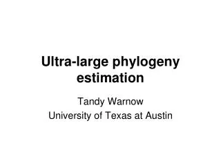
Estimating Ultra-large Phylogenies and Alignments Tandy Warnow Department of Computer Science The University of Texas at Austin
How did life evolve on earth? • Courtesy of the Tree of Life project NP-hard optimization problems Stochastic models of evolution Statistical methods Statistical performance issues Millions of taxa Important applications Current projects (e.g., iPlant) will attempt to estimate phylogenies with upwards of 500,000 species
-3 mil yrs AAGACTT AAGACTT -2 mil yrs AAGGCCT AAGGCCT AAGGCCT AAGGCCT TGGACTT TGGACTT TGGACTT TGGACTT -1 mil yrs AGGGCAT AGGGCAT AGGGCAT TAGCCCT TAGCCCT TAGCCCT AGCACTT AGCACTT AGCACTT today AGGGCAT TAGCCCA TAGACTT AGCACAA AGCGCTT AGGGCAT TAGCCCA TAGACTT AGCACAA AGCGCTT DNA Sequence Evolution
U V W X Y AGGGCAT TAGCCCA TAGACTT TGCACAA TGCGCTT X U Y V W
Current Research Projects Method development: • Large-scale multiple sequence alignment and phylogeny estimation • Metagenomics • Comparative genomics • Estimating species trees from gene trees • Supertree methods • Phylogenetic estimation under statistical models Dataset analyses (multi-institutional collaborations): • Avian Phylogeny (and brain evolution) • Human Microbiome • Thousand Transcriptome (1KP) Project • Conifer evolution
SATé: Simultaneous Alignment and Tree Estimation (Liu et al., Science 2009, and Liu et al. Systematic Biology, in press) • DACTAL: Divide-and-Conquer Trees without alignments (Nelesen et al., in preparation) • SEPP: SATé-enabled Phylogenetic Placement (Mirarab, Nguyen, and Warnow, PSB 2012, in press)
Part 1: SATé Liu, Nelesen, Raghavan, Linder, and Warnow, Science, 19 June 2009, pp. 1561-1564. Liu et al., Systematic Biology (in press)
U V W X Y TAGACTT TGCACAA TGCGCTT AGGGCATGA AGAT X U Y V W
Deletion Substitution …ACGGTGCAGTTACCA… • The true multiple alignment • Reflects historical substitution, insertion, and deletion events • Defined using transitive closure of pairwise alignments computed on edges of the true tree Insertion …ACGGTGCAGTTACC-A… …AC----CAGTCACCTA… …ACCAGTCACCTA…
Input: unaligned sequences S1 = AGGCTATCACCTGACCTCCA S2 = TAGCTATCACGACCGC S3 = TAGCTGACCGC S4 = TCACGACCGACA
Phase 1: Multiple Sequence Alignment S1 = AGGCTATCACCTGACCTCCA S2 = TAGCTATCACGACCGC S3 = TAGCTGACCGC S4 = TCACGACCGACA S1 = -AGGCTATCACCTGACCTCCA S2 = TAG-CTATCAC--GACCGC-- S3 = TAG-CT-------GACCGC-- S4 = -------TCAC--GACCGACA
Phase 2: Construct tree S1 = AGGCTATCACCTGACCTCCA S2 = TAGCTATCACGACCGC S3 = TAGCTGACCGC S4 = TCACGACCGACA S1 = -AGGCTATCACCTGACCTCCA S2 = TAG-CTATCAC--GACCGC-- S3 = TAG-CT-------GACCGC-- S4 = -------TCAC--GACCGACA S1 S2 S4 S3
Phylogeny methods Bayesian MCMC Maximum parsimony Maximum likelihood Neighbor joining FastME UPGMA Quartet puzzling Etc. Two-phase estimation Alignment methods • Clustal • POY (and POY*) • Probcons (and Probtree) • Probalign • MAFFT • Muscle • Di-align • T-Coffee • Prank (PNAS 2005, Science 2008) • Opal (ISMB and Bioinf. 2007) • FSA (PLoS Comp. Bio. 2009) • Infernal (Bioinf. 2009) • Etc. RAxML: heuristic for large-scale ML optimization
S1 S1 S2 S4 S4 S2 S3 S3 Simulation Studies S1 = AGGCTATCACCTGACCTCCA S2 = TAGCTATCACGACCGC S3 = TAGCTGACCGC S4 = TCACGACCGACA Unaligned Sequences S1 = -AGGCTATCACCTGACCTCCA S2 = TAG-CTATCAC--GACCGC-- S3 = TAG-CT-------GACCGC-- S4 = -------TCAC--GACCGACA S1 = -AGGCTATCACCTGACCTCCA S2 = TAG-CTATCAC--GACCGC-- S3 = TAG-C--T-----GACCGC-- S4 = T---C-A-CGACCGA----CA Compare True tree and alignment Estimated tree and alignment
Quantifying Error FN FN: false negative (missing edge) FP: false positive (incorrect edge) 50% error rate FP
Problems with the two-phase approach • Current alignment methods fail to return reasonable alignments on large datasets with high rates of indels and substitutions. • Manual alignment is time consuming and subjective. • Potentially useful markers are often discarded if they are difficult to align. These issues seriously impact large-scale phylogeny estimation (and Tree of Life projects)
Obtain initial alignment and estimated ML tree Tree SATé Algorithm
Obtain initial alignment and estimated ML tree Tree Use tree to compute new alignment Alignment SATé Algorithm
Obtain initial alignment and estimated ML tree Tree Use tree to compute new alignment Estimate ML tree on new alignment Alignment SATé Algorithm
Obtain initial alignment and estimated ML tree Tree Use tree to compute new alignment Estimate ML tree on new alignment Alignment SATé Algorithm If new alignment/tree pair has worse ML score, realign using a different decomposition Repeat until termination condition (typically, 24 hours)
A C A B Decompose based on input tree C D B D Align subproblems A B C D Estimate ML tree on merged alignment ABCD Merge subproblems One SATé iteration (really 32 subsets) e
1000 taxon models, ordered by difficulty 24 hour SATé analysis, on desktop machines (Similar improvements for biological datasets)
Understanding SATé • Observations: (1) subsets of taxa that are small enough, closely related, and densely sampled are aligned more accurately than others. • SATé-1 produces subsets that are closely related and densely sampled, but not small enough. • SATé-2 (“next SATé”) changes the design to produce smaller subproblems. • The next iteration starts with a more accurate tree. This leads to a better alignment, and a better tree.
Software In use by research groups around the world • Kansas SATé software developers: Mark Holder, Jiaye Yu, and Jeet Sukumaran • Downloadable software for various platforms • Easy-to-use GUI • http://phylo.bio.ku.edu/software/sate/sate.html
A C B D Limitations of SATé-I and -II A B Decompose dataset C D Align subproblems A B C D Estimate ML tree on merged alignment ABCD Merge sub-alignments
Part II: DACTAL(Divide-And-Conquer Trees (without) ALignments) • Input: set S of unaligned sequences • Output: tree on S (but no alignment) (Nelesen, Liu, Wang, Linder, and Warnow, in preparation)
DACTAL BLAST-based Existing Method: RAxML(MAFFT) Unaligned Sequences Overlapping subsets pRecDCM3 A tree for each subset New supertree method: SuperFine A tree for the entire dataset
Average of 3 Largest CRW Datasets CRW: Comparative RNA database, datasets 16S.B.ALL, 16S.T, and 16S.3 6,323 to 27,643 sequences These datasets have curated alignments based on secondary structure Reference trees are 75% RAxML bootstrap trees DACTAL (shown in red) run for 5 iterations starting from FT(Part) DACTAL is robust to starting trees PartTree and Quicktree are the only MSA methods that run on all 3 datasets FastTree (FT) and RAxML are ML methods
DACTAL outperforms SATé • DACTAL faster and matches or improves upon accuracy of SATé for datasets with 1000 or more taxa • The biggest gains are on the very large datasets
Part III: SEPP • SEPP: SATé-enabled Phylogenetic Placement, by Mirarab, Nguyen, and Warnow • To appear, Pacific Symposium on Biocomputing, 2012 (special session on the Human Microbiome)
Metagenomic data analysis NGS data produce fragmentary sequence data Metagenomic analyses include unknown species Taxon identification: given short sequences, identify the species for each fragment Applications: Human Microbiome Issues: accuracy and speed
Phylogenetic Placement Input: Backbone alignment and tree on full-length sequences, and a set of querysequences (short fragments) Output: Placement of query sequences on backbone tree Phylogenetic placement can be used for taxon identification, but it has general applications for phylogenetic analyses of NGS data.
Phylogenetic Placement Align each query sequence to backbone alignment Place each query sequence into backbone tree, using extended alignment
Align Sequence S1 = -AGGCTATCACCTGACCTCCA-AA S2 = TAG-CTATCAC--GACCGC--GCA S3 = TAG-CT-------GACCGC--GCT S4 = TAC----TCAC--GACCGACAGCT Q1 = TAAAAC S1 S2 S3 S4
Align Sequence S1 = -AGGCTATCACCTGACCTCCA-AA S2 = TAG-CTATCAC--GACCGC--GCA S3 = TAG-CT-------GACCGC--GCT S4 = TAC----TCAC--GACCGACAGCT Q1 = -------T-A--AAAC-------- S1 S2 S3 S4
Place Sequence S1 = -AGGCTATCACCTGACCTCCA-AA S2 = TAG-CTATCAC--GACCGC--GCA S3 = TAG-CT-------GACCGC--GCT S4 = TAC----TCAC--GACCGACAGCT Q1 = -------T-A--AAAC-------- S1 S2 S3 S4 Q1
Phylogenetic Placement • Align each query sequence to backbone alignment • HMMALIGN (Eddy, Bioinformatics 1998) • PaPaRa (Berger and Stamatakis, Bioinformatics 2011) • Place each query sequence into backbone tree • Pplacer (Matsen et al., BMC Bioinformatics, 2011) • EPA (Berger and Stamatakis, Systematic Biology 2011) Note: pplacer and EPA use maximum likelihood
HMMER vs. PaPaRa Alignments 0.0 Increasing rate of evolution
SEPP Parameter Exploration Alignment subset size and placement subset size impact the accuracy, running time, and memory of SEPP 10% rule (subset sizes 10% of backbone) had best overall performance
SEPP (10%-rule) on simulated data 0.0 0.0 Increasing rate of evolution
SEPP (10%) on Biological Data 16S.B.ALL dataset, 13k curated backbone tree, 13k total fragments
SEPP (10%) on Biological Data 16S.B.ALL dataset, 13k curated backbone tree, 13k total fragments For 1 million fragments: PaPaRa+pplacer: ~133 days HMMALIGN+pplacer: ~30 days SEPP 1000/1000: ~6 days