Download
1 / 40
420 likes | 599 Views
Confounding 混杂偏倚. Michael Engelgau Shanghai FETP August 15, 2012. The Nature of Epidemiologic Research. Epidemiology is the study of disease occurrence and health indicators in human populations

E N D
Confounding混杂偏倚 Michael Engelgau Shanghai FETPAugust 15, 2012
The Nature of Epidemiologic Research • Epidemiology is the study of disease occurrence and health indicators in human populations • The use of populations distinguishes epidemiology from other biomedical sciences and clinical medicine • Basic features of population epidemiology: • Quantitative/empirical • Probabilistic • Comparative
Causal Inference in Epidemiology Bridging the gap between our ideas and our observations. Criteria: • Strength of association • Consistency of findings • Specificity of association • Temporality (lack of ambiguity) • Biologic gradient (dose-response effect) • Biologic plausibility of the hypothesis • Coherence of evidence • Experimental evidence
Confounding: A Fundamental Problem of Causal Inference • Confounding is bias due to inherent (unobservable) differences in risk between exposed and unexposed populations, i.e., a lack of comparability. • Confounding is usually not a major source of bias in randomized trials (assuming sample size is large enough) because randomization tends to equalize inherent risks between treatment groups (treated group = exposed, untreated = unexposed)
Confounding • May lead to observation of association when none exists • May obscure an association that exists • Information on potential confounders should be collected in the study and used in analysis, otherwise they cannot be excluded as alternate explanations for findings • Confounding factors must be considered during study design
Confounding • Mixing of the effect of the exposure on disease with the effect of another factor that is associated with the exposure • Bias in estimating the effect of exposure (E) on disease (D) occurrence, due to the lack of comparability between exposed and unexposed populations • Risk among exposed ≠ Risk among exposed if they had been unexposed
Confounding • We cannot directly examine the correctness of the comparability assumption that defines confounding (presence or absence of confounding cannot be observed because it depends on a counterfactual condition: risk in the exposed group in the absence of exposure) • Instead we attempt to identify and control for empirical manifestations of confounding.
Properties of Confounders 3 Criteria for a variable to be a confounder (C): • C must be a risk factor for the disease (D) in the unexposed population • C must be associated with exposure (E) in the population from which the cases arose • The association between C and E must not be due entirely to the effect of E on C (meaning C cannot be an intermediate step between E and D)
EXPOSURE DISEASE
EXPOSURE DISEASE CONFOUNDER
INTERMEDIATE EXPOSURE DISEASE CONFOUNDER
Example of Confounding Alcohol drinking Oral cancer Potential Confounders
Example of Confounding Alcohol drinking Oral cancer Cigarette smoking
Example of Confounding Birth order Down Syndrome Potential Confounders
Second, third and fourth child are more often affected by Down Syndrome than the first child
Example of Confounding Birth Order Down Syndrome Maternal Age
Confounding or Intermediate Effect? • If a covariate is an intermediate variable (I) in the causal pathway linking E and D, then conventional adjustment for this variable will produce a biased estimate of the net E effect. • Typically, the direction of this bias will be toward the null (no effect). • The process of executing sophisticated statistical modeling is, at times, divorced from making sound causal inference.
Confounding or Intermediate Effect? • Researchers should carefully scrutinize each variable considered for adjustment in an attempt to report unbiased estimates of the effect of exposure. • Bulterys & Morgenstern proposed the term “iatrogenic bias” to denote bias introduced by the analyst when inappropriately controlling for variables as though they were confounders (Paediatr Perinat Epidemiol 1993; 7:387-94).
Confounding or Intermediate Effect? • The process of covariate adjustment depends critically on the investigator’s prior knowledge of disease etiology and on adequate resources for measuring confounders accurately. • Graphical examination of the relationships among 3 or more variables useful. • Alternative, more complex analytic approaches such as G-estimation (Robins JM et al.) may also be used.
Confounding or Intermediate Effect? Physical Activity Colorectal Cancer Body Mass Index Obesity ?
Confounding and/or Intermediate Effect? • In many instances, it may be most appropriate to present both adjusted and unadjusted estimates of effect. Thus, readers can assess the sensitivity of conclusions to alternative assumptions about the possible effect of the exposure on certain covariates. • CAN YOU THINK OF EXAMPLES?
Residual Confounding • If a confounding variable is misclassified, the ability to control confounding in the analysis is hampered. • If confounding is strong and the E – D relation is weak, misclassification of the confounding variable can lead to very misleading results. • Residual confounding occurs when adjustment is not sufficiently fine to take into account the full variability of the outcome. Example: adjusting for smoking history using a crude ever/never variable vs. using detailed smoking duration or age began smoking.
Heterogeneity in measure of effect across levels of a third variable • Identify a subgroup with a lower or higher risk to study interaction between risk factors, and to target public health action Effect Measure Modification
HIV prevalence and age difference in years between pregnant women and spouse/partner, Zambia, 2004
HIV prevalence and age difference in years between pregnant women and spouse/partner, Zambia, 2004
Controlling Confounding In the design • Restrict the study population • Matching • Collect information on potential confounders In the analysis • Control for confounding through • Restrict the analysis to subgroups • Stratified analysis • Multivariable regression
Restriction Restrict the study or the analysis to a subgroup that is homogenous for the possible confounder.
Evaluation of Confounding and Effect Modification by Stratification • Consider potential confounders and effect measure modifiers • Stratify by levels of potential confounder or modifiers • Compute stratum specific measures of association (OR or RR) • Evaluate similarity of stratum specific estimates (test for homogeneity) • If stratum specific estimates are similar, then calculate summary adjusted estimate • Evaluate change in estimate between crude and adjusted estimates (5%, 10%, 20%) • If the effect are not uniform, and are statistically different, then report stratum specific estimates
Adjusting for Confounding: Stratified Analysis Strengths • Ease and clarity of presentation • Mantel-Haenszel method combines subgroups to provide a summary Weaknesses • Small numbers in the subgroups • Adjusts for only one variable (the stratum)
Adjusting for Confounding: Multivariate Analysis • Analyze data in a statistical model that includes both the presumed cause (exposure) and possible confounders • Determine a priori the criteriafor inclusion of covariates in the model (prior knowledge, change in estimate) • Evaluate the independent effect of an exposure after adjustment for other measured confounders
Multivariate Analysis Strengths • Can adjust for multiple covariates simultaneously Weaknesses • Subjects with missing data on covariates are deleted from analysis, may lead to biased results • Sophisticated process requires valid assumptions on which the model is based. • Results can be difficult to display or explain to inexperienced readers
Limitations of Regression Modeling • The logistic regression model and the Cox proportional hazards model are most commonly used. Both models are based on similar assumptions (e.g., joint effects are multiplicative). • Selection of variables in the model should be based primarily on prior knowledge of relevant associations. • Liberal use of graphical methods is recommended for checking the reasonableness of model assumptions. • Model-based results should always be subjected to sensitivity analyses.
Model Building Terms in the model Model colorectal cancer = Physical activity 0.60 (0.44-0.83) Model colorectal cancer = Body mass index 6.31 (1.55-25.70) Model colorectal cancer = Age + physical activity 0.64 (0.42-0.96) Model colorectal cancer = Age + physical activity + body mass index 0.73 (0.52-1.01)
Model Building Terms in the model Model colorectal cancer = Physical activity 0.60 (0.44-0.83) Model colorectal cancer = Age + physical activity 0.64 (0.42-0.96) (0.64 – 0.60) = 0.04; (0.04/0.60 x 100) = 6.7% Model colorectal cancer = Age + physical activity + body mass index 0.73 (0.52-1.01) (0.73 – 0.64) = .09; (0.09/0.64 x 100) = 14.1%
MET-hours per week – year before enrollmentColon cancer, men Terms in model Highest vs. lowest Age 0.64 (0.42-0.96) Age + education 0.67 (0.45-1.02) Age + family history 0.64 (0.42-0.96) Age + BMI 0.69 (0.46-1.04) Age + energy 0.64 (0.42-0.96) Age + occupation 0.64 (0.43-0.97) Age + cigarette smoking 0.65 (0.43-0.98) Age + alcohol 0.64 (0.43-0.97) Age + aspirin 0.64 (0.43-0.97) Age + multivitamin use 0.65 (0.43-0.97) Age + fiber 0.68 (0.45-1.03) Age + folate 0.67 (0.45-1.02) Age + calcium 0.66 (0.43-0.99) Age + red meat 0.66 (0.44-0.99) Age + vegetables 0.67 (0.44-1.01) Age + fruit 0.66 (0.44-1.00) Age + hours spent sitting 0.63 (0.42-0.95)
Further Reading • Modern Epidemiology (3rd Edition). Eds: K. Rothman, S. Greenland, T Lash. Lippincott et al, 2008. [chapters 2, 9, 12, 21 & 26] • Rothman KJ, Greenland S. Causation and causal inference in epidemiology. Am J Public Health 2005; 95:S144-S150. • Greenland S, Morgenstern H. Confounding in health research. Annu Rev Public Health 2001; 22:189-212. • Special thanks to Drs. Bob Fontaine and Marc Bulterys.
Modify what you wrote down: - What is the research question (issue)? - What is/are the outcome(s) or disease(s)? - What is/are the exposure(s)? - What’s the study population? Where? Age? - What data will you collect? What variables? - How will you collect the data? - What analyses will you perform? - What manuscripts will you generate? Exercise

![Religion and natural philosophy [“science”] in earth studies* Cosmogonies Chronologies Natural theology](https://cdn0.slideserve.com/6206/slide1-dt.jpg)