Download
1 / 73
740 likes | 877 Views
Novel Approaches to Adjusting for Confounding: Propensity Scores, Instrumental Variables and MSMs. Matthew Fox Advanced Epidemiology. What are the exposures you are interested in studying?.

E N D
Novel Approaches to Adjusting for Confounding:Propensity Scores, Instrumental Variables and MSMs Matthew Fox Advanced Epidemiology
Assuming I could guarantee you that you would not create bias, which approach is better: randomization or adjustment for every known variable?
Yesterday • Causal diagrams (DAGS) • Discussed rules of DAGS • Goes beyond statistical methods and forces us to use prior causal knowledge • Teaches us adjustment can CREATE bias • Helps identify a sufficient set of confounders • Not how to adjust for them
This week • Beyond stratification and regression • New approaches to adjusting for (not “controlling” ) confounding • Instrumental variables • Propensity scores (Confounder scores) • Marginal structural models • Time dependent confounding
Given the problems with the odds ratio, why does everyone use it?
Solution: SAS Code title "Crude relative risk model"; procgenmod data=odds descending; model d = e/link=log dist=bin; run; title "Adjusted relative risk model"; procgenmod data=odds descending; model d = e c/link=log dist=bin; run;
Results Model crude: Exp(0.5288) = 1.6968 Crude RR was 1.6968
Results Model adjusted: Exp(0.3794) = 1.461 MH RR was 1.55
STATA • glm d e, family(binomial) link(log) • glm d e c, family(binomial) link(log)
Solution: SAS Code title "Crude risk differences model"; procgenmod data=odds descending; model d = e/link=bin dist=identity; run; title "Adjusted risk differences model"; procgenmod data=odds descending; model d = e c/link=bin dist=identity; run;
Results Model crude: 0.239 Crude RD = 0.23896 Model crude: Exp(0.5288) = 1.6968 Crude RR was 1.7
Results Adjusted model : 0.20 MH RD = 0.20
STATA • glm d e, family(binomial) link(identity) • glm d e c, family(binomial) link(identity) • glm d e c c*e, family(binomial) link(identity)
Limitations of Stratification and Regression • Stratification/regression work well with point exposures with complete follow up and sufficient data to adjust • Limited data on confounders or small cells • No counterfactual for some people in our dataset • Regression often estimates parameters • Time dependent exposures and confounding • A common situation • With time dependence, DAGs gets complex
Randomization and Counterfactuals • Ideally, evidence comes from RCTs • Randomization gives expectation unexposed can stand in for the counterfactual ideal • Full exchangeability: E(p1=q1, p2=q2, p3=q3, p4=q4) • In expectation, assuming no other bias • [Pr(Ya=1=1) - Pr(Ya=0=1)] = [Pr(Y=1|A=1) - Pr(Y=1|A=0)] • Since we assign A, RRAC = 1 • If we can’t randomize, what can we do to approximate randomization?
How randomization works Randomized Controlled Trial C1 C2 C3 Randomization A D Randomization strongly predicts exposure (ITT)
A typical observational study Observational Study C1 C2 C3 ? A D
A typical observational study Observational Study C1 C2 C3 A D Regression/stratification seeks to block backdoor path from A to D by averaging A-D associations within levels of Cx
Intention to treat analysis • In an RCT we assign the exposure • e.g. assign people to take an aspirin a day vs. not • But not all will take aspirin when told to and others will take it even if told not to • What to do with those who don’t “obey”? • The paradigm of intention to treat analysis says analyze subject in the group they are assigned • Maintains the benefits of randomization • Biases towards the null at worst
Instrumental variables • An approach to dealing with confounding using a single variable • Works along the same lines as randomization • Commonly used approach in economics, yet rarely used in medical research • Suggests we are either behind the times or they are hard to find • Party privileged in economics because little adjustment data exists
Instrumental variables • An instrument (I): • A variable that satisfies 3 conditions: • Strongly associated with exposure • Has no effect on outcome except through A (E) • Shares no common causes with outcome • Ignore E-D relationship • Measure association between I and D • This is not confounded • Approximates an ITT approach
Adjust the IV estimate • Can optionally adjust IV estimate to estimate the effect of A (exposure) • But differs from randomization • If an instrument can be found, has the advantage we can adjust for unknown confounders • This is the benefit we get from randomization?
Intention to Treat (IV Ex 1) • A(Exposure): Aspirin vs. Placebo • Outcome: First MI • Instrument: Randomized assignment Condition 1: Predictor of A ? Condition 2: no direct effect on the outcome? Condition 3: No common causes with outcome? Confounders Randomization Therapy MI
Regression (17 confounders), no effect RD: -0.06/100; 95% CI -0.26 to 0.14 IV: Protective effect of COX-2 RD: -1.31/100; -2.42 to -0.20 Compatible with trial results RD: -0.65/100; -1.08 to -0.22 Confounding by indication (IV Ex 2) • A(Exposure): COX2 inhibitor vs NSAID • Outcome: GI complications • Instrument: Physician’s previous prescription Indications Previous Px COX2/NSAID GI comp
For 3,964 women born 1919-1940, a 1 SD (1.3 ºC) > mean summer temp in 1st year life associated with 1.12-mmHg (95% CI: 0.33, 1.91) > adult systolic blood pressure, and 1 SD > mean summer rainfall (33.9 mm) associated with < systolic blood pressure (-1.65 mmHg, 95% CI: -2.44, -0.85). Unknown confounders (IV Ex 3) • A(Exposure): Childhood dehydration • Outcome: Adult high blood pressure • Instrument: 1st year summer climate Hypothesized hottest/driest summers in infancy would be associated with severe infant diarrhea/dehydration, and consequently higher blood pressure in adulthood. SES 1st year climate dehydration High BP
Optionally we can adjust for “non-compliance” • Optionally if we want to estimate A-D relationship, not I-D, we can adjust: • RDID / RDIE • Inflate the IV estimator to adjust for the lack of perfect correlation between I and E • If I perfectly predicts E then RDIE = 1, so adjustment does nothing • Like per protocol analysis • But adjusted for confounders
To good to be true? • Maybe • The assumptions needed for an instrument are un-testable from the data • Can only determine if I is associated with A • Failure to meet the assumptions can cause strong bias • Particularly if we have a “weak” instrument
Comes out of a world of large datasets (Health insurance data) • Cases where we have a small (relative to the size of the dataset) exposed population and lots and lots of potential comparisons in the unexposed group • And lots of covariate data to adjust for • Then we have luxury of deciding who to include in study as a comparison group based on a counterfactual definition
Propensity Score • Model each subject’s propensity to receive the index condition as a function of confounders • Model is independent of outcomes, so good for rare disease, common exposure • Use the propensity score to balance assignment to index or reference by: • Matching • Stratification • Modeling
Propensity Scores • The propensity score for subject i is: • Probability of being assigned to treatment A = 1 vs. reference A = 0 given a vector xi of observed covariates: • In other words, the propensity score is: • Probability that the person got the exposure given anything else we know about them
Why estimate the probability a subject receives a certain treatment when it is known what treatment they received?
Quasi-experiment Using probability a subject would have been treated (propensity score) to adjust estimate of the treatment effect, we simulate a RCT 2 subjects with = propensity, one E+, one E- We can think of these two as “randomly assigned” to groups, since they have the same probability of being treated, given their covariates Assumes we have enough observed data that within levels of propensity E is truly random How Propensity Scores Work
Have info on people’s covariates: Alcohol use, sex, weight, age, exercise, etc: Person A is a smoker, B is not Both had 85% predicted probability of smoking If “propensity” to smoke is same, only difference is 1 smoked and 1 didn’t This is essentially what randomization does B is the counterfactual for A assuming a correct model for predicting smoking Propensity Scores:Smoking and Colon Cancer
Calculate propensity score proc logistic; model exposure = cov_1 cov_2 … cov_n; output out = pscoredat pred = pscore; run; Either match subjects on propensity score or adjust for propensity score proc logistic; model outcome = exposure pscore; run; Obtaining Propensity Scores in SAS
Pros and Cons of PS • Pros • Adjustment for 1 confounder • Allows estimation of the exposure and fitting a final model without ever seeing the outcome • Allows us to see parts of data we really should not be drawing conclusions on b/c no counterfactual • Cons • Only works if have good overlap in pscores • Does not fix conditioning on a collider problem • Doesn’t deal with unmeasured confounders
Time Dependent Confounding • Time dependent confounding: • Time dependent covariate that is a risk factor for or predictive of the outcome and also predicts subsequent exposure • Problematic if also: • Past exposure history predicts subsequent level of covariate
Example • Observational study of subjects infected with HIV • E = HAART therapy • D = All cause mortality • C = CD4 count
Time Dependent Confounding A0 A1 D 1) C0 C1 A0 A1 D 2) C0 C1
Failure of Traditional Methods • Want to estimate causal effect of A on D • Can’t stratify on C (it’s an intermediate) • Can’t ignore C (it’s a confounder) • Solution – rather than stratify, weight • Equivalent to standardization • Create pseudo-population where RRCE = 1 • Weight each person by “inverse probability of treatment” they actually received • Weighting doesn’t cause problems pooling did • In DAG, remove arrow C to A, don’t box